Spatial IsoDepth Calculation

GASTON is an interpretable deep learning model for learning the gene expression topography of a tissue slice from spatially resolved transcriptomics (SRT) data. GASTON models gene expression topography by learning the isodepth, a 1-D coordinate describing continuous gene expression gradients and tissue geometry (i.e. spatial domains).

Here, we introduce method integrated in omicverse named GASTON.

We made three improvements in integrating the GASTON algorithm in OmicVerse:

• We reduced the installation conflict of GASTON, user only need to update OmicVerse to the latest version.

• We optimized the visualization of GASTON and simplify the function input of GASTON.

• We have fixed some bugs that could occur during function.

Besides, all functions you could find in omicverse.external.GASTON if you want to use the raw functuion to run GASTON’s tutorial

import omicverse as ov
#print(f"omicverse version: {ov.__version__}")
import scanpy as sc
#print(f"scanpy version: {sc.__version__}")
ov.plot_set()

Warning: Could not read dependencies from pyproject.toml: [Errno 2] No such file or directory: '/home/groups/xiaojie/steorra/env/omicverse/lib/python3.10/site-packages/omicverse/pyproject.toml'

   ____            _     _    __                  
  / __ \____ ___  (_)___| |  / /__  _____________ 
 / / / / __ `__ \/ / ___/ | / / _ \/ ___/ ___/ _ \ 
/ /_/ / / / / / / / /__ | |/ /  __/ /  (__  )  __/ 
\____/_/ /_/ /_/_/\___/ |___/\___/_/  /____/\___/                                              

Version: 1.6.11, Tutorials: https://omicverse.readthedocs.io/

Prepared stRNA-seq

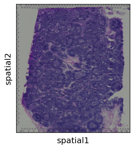
First let’s read spatial Visium data from 10X Space Ranger output. Here we use lymph node data generated by 10X and presented in Kleshchevnikov et al (section 4, Fig 4). This dataset can be conveniently downloaded and imported using scanpy. See this tutorial for a more extensive and practical example of data loading (multiple visium samples).

adata = sc.datasets.visium_sge(sample_id="V1_Human_Lymph_Node")
adata

reading /scratch/users/steorra/analysis/omicverse/omicverse_guide/docs/Tutorials-space/data/V1_Human_Lymph_Node/filtered_feature_bc_matrix.h5
 (0:00:01)

AnnData object with n_obs × n_vars = 4035 × 36601
    obs: 'in_tissue', 'array_row', 'array_col'
    var: 'gene_ids', 'feature_types', 'genome'
    uns: 'spatial'
    obsm: 'spatial'

adata.var_names_make_unique()
adata.obs_names_make_unique()

sc.pl.spatial(adata,
             color=None,
             show=False)

[<AxesSubplot: xlabel='spatial1', ylabel='spatial2'>]

Use top PCs of analytic Pearson residuals

Here we compute PCA on analytic Pearson residuals following the Scanpy tutorial https://scanpy-tutorials.readthedocs.io/en/latest/tutorial_pearson_residuals.html tutorial . This is faster than GLM-PCA, but the PCs are of lower quality, so it is not recommended

gas_obj=ov.space.GASTON(adata)
gas_obj.get_gaston_input(get_rgb=True,spot_umi_threshold=50)
A=gas_obj.get_top_pearson_residuals(num_dims=8,clip=0.01,n_top_genes=5000,
                                 use_RGB=True)

filtered out 1 cells that have less than 50 counts
Adding image layer `img1`
calculating RGB
Calculating features `['summary']` using `1` core(s)
Adding `adata.obsm['features']`
Finish (0:00:30)
extracting highly variable genes
--> added
    'highly_variable', boolean vector (adata.var)
    'highly_variable_rank', float vector (adata.var)
    'highly_variable_nbatches', int vector (adata.var)
    'highly_variable_intersection', boolean vector (adata.var)
    'means', float vector (adata.var)
    'variances', float vector (adata.var)
    'residual_variances', float vector (adata.var)
normalizing counts per cell
    finished (0:00:00)
computing analytic Pearson residuals on adata.X
    finished (0:00:00)
computing PCA
    with n_comps=8
    finished (0:00:00)

We first load GLM-PCs and coordinates and z-score normalize.

gas_obj.load_rescale(A)

Training the GASTON model

Next we train the neural network, once for each random initialization.

NEURAL NET PARAMETERS (USER CAN CHANGE) architectures are encoded as list, eg [20,20] means two hidden layers of size 20 hidden neurons

• isodepth_arch: architecture for isodepth neural network d(x,y) : R^2 -> R

• expression_fn_arch: architecture for 1-D expression function h(w) : R -> R^G

• num_epochs: number of epochs to train NN (NOTE: it is sometimes beneficial to train longer)

• checkpoint: save model after number of epochs = multiple of checkpoint

• out_dir: folder to save model runs

• optimizer:

• num_restarts=20

out_dir='/scratch/users/steorra/tmp/tmp'
gas_obj.train(
    isodepth_arch=[20,20],
    expression_fn_arch=[20,20],
    num_epochs=5000,
    checkpoint=500,
    out_dir=out_dir,
    optimizer="adam",
    num_restarts=20
)

Visualization

If you use the model trained above, then figures will closely match the manuscript — but not exactly match — due to PyTorch non-determinism in seeding (see https://github.com/pytorch/pytorch/issues/7068 ).

We also include the model used in the paper for reproducibility.

out_dir='/scratch/users/steorra/tmp/tmp'
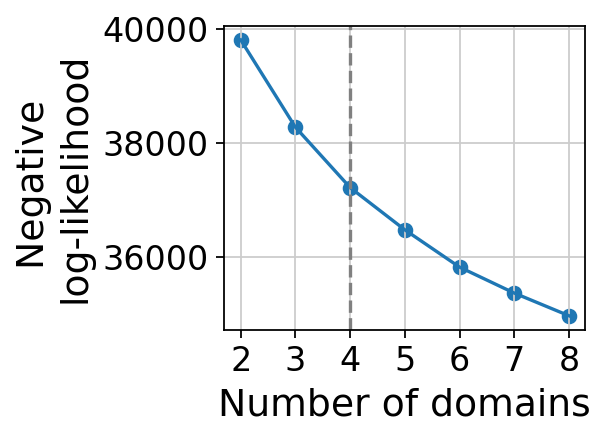
gaston_model, A, S=gas_obj.get_best_model(out_dir=out_dir,
                       max_domain_num=8,start_from=2)

best model: /scratch/users/steorra/tmp/tmp/rep9
Kneedle number of domains: 4

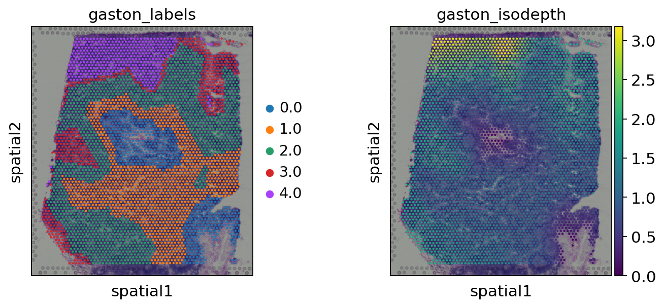
Calculate the IsoDepth and Labels

We can chose the number of layers from IsoDepth

gaston_isodepth, gaston_labels=gas_obj.cal_iso_depth(5)

adata.obs['gaston_labels']=[str(i) for i in gaston_labels]
adata.obs['gaston_isodepth']=gaston_isodepth

sc.pl.spatial(adata,
             color=['gaston_labels','gaston_isodepth'],
             show=False)

[<AxesSubplot: title={'center': 'gaston_labels'}, xlabel='spatial1', ylabel='spatial2'>,
 <AxesSubplot: title={'center': 'gaston_isodepth'}, xlabel='spatial1', ylabel='spatial2'>]

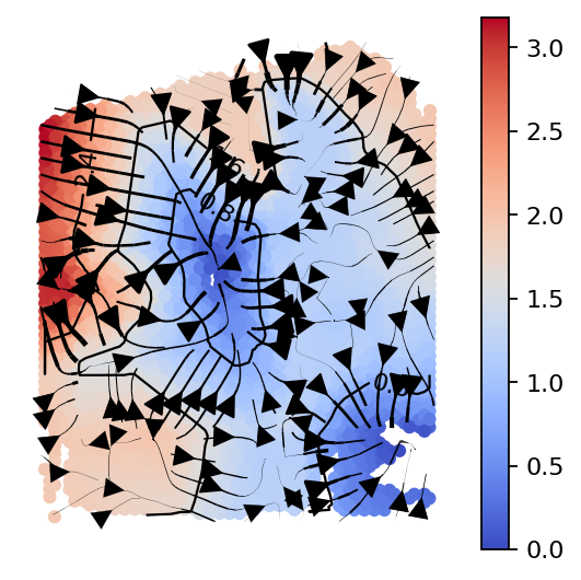
gas_obj.plot_isodepth(show_streamlines=True,
                      rotate_angle=-90,arrowsize=2,
                      figsize=(4,4),n_neighbors=100)

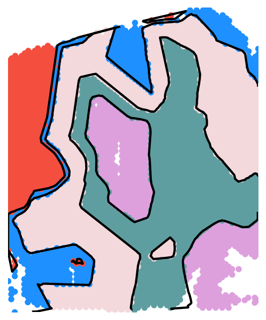
domain_colors=['plum', 'cadetblue', '#F3D9DC','dodgerblue', '#F44E3F']
gas_obj.plot_clusters(
    domain_colors,
    boundary_lw=2,
    figsize=(4,5),
    rotate_angle=-90,
)

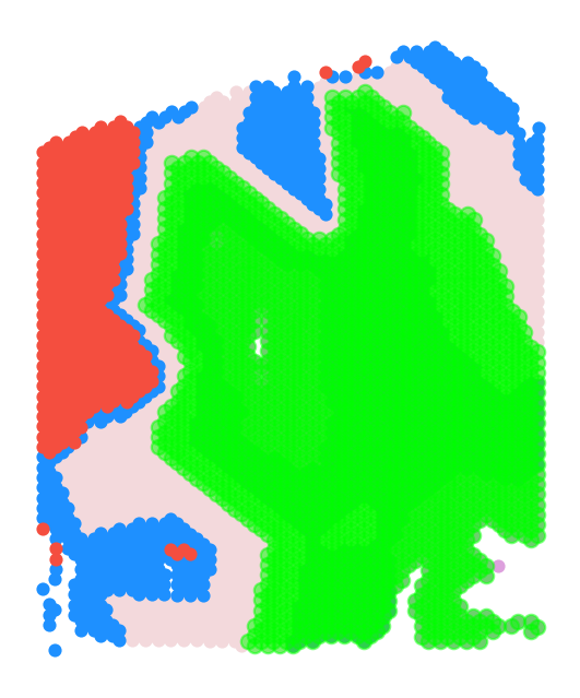
Specific to this analysis: restrict to domains (0,1)

To isolate the tumor section, we restrict to spots with isodepth lying in a given range. The range of isodepth values will need to be tuned depending on the specific application.

In some cases, the tissue geometry cannot be represented with a single isodepth. In this case, we recommend first subsetting your tissue to the specific region of interest (eg from ScanPy clustering), and then running GASTON

gas_obj.plot_clusters_restrict(
    domain_colors,
    isodepth_min=0,
    isodepth_max=1.5,
    rotate_angle=-90,
    s=20,lgd=False,
    figsize=(4,5)
)

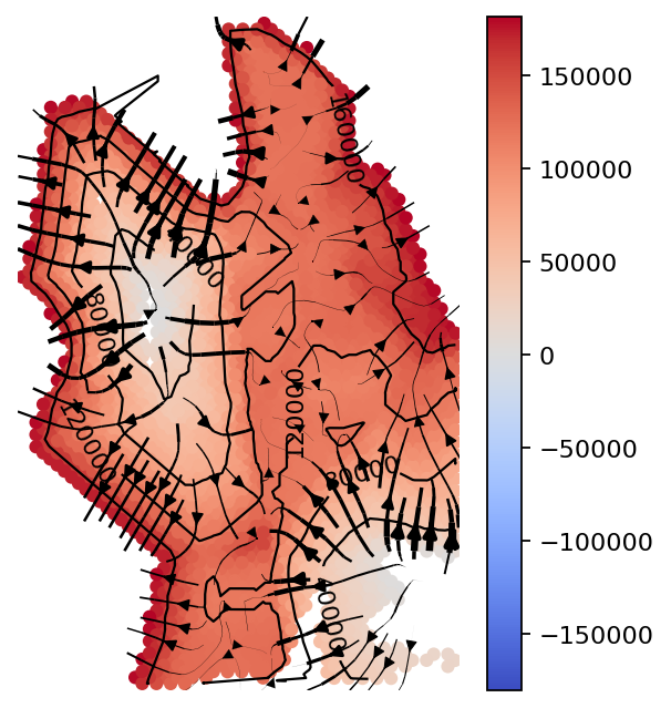
counts_mat_restrict, coords_mat_restrict, gaston_isodepth_restrict, gaston_labels_restrict, S_restrict=gas_obj.restrict_spot(
    isodepth_min=0,
    isodepth_max=1.5,
    adjust_physical=True,
    scale_factor=100,
    plotisodepth=True,
    show_streamlines=True,
    rotate_angle=-90,
    arrowsize=1, figsize=(4,5), 
    neg_gradient=True,
    n_neighbors=500
)

restricting to 2280 spots

gas_obj.filter_genes(
    umi_thresh = 1000,
    exclude_prefix=['MT-', 'RPL', 'RPS']
)

pw_fit_dict=gas_obj.pw_linear_fit()
binning_output=gas_obj.bin_data(
    num_bins=15,
    q_discont=0.95,
    q_cont=0.8
)

The binning_output, cont_genes_layer and discont_genes_layer stored in gas_obj

ad=gas_obj.get_restricted_adata(gas_obj,offset=10**6)

Plot discontinuous and continuous genes

We can found the discontinuous genes using gas_obj.discont_genes_layer and found continuous genes using gas_obj.cont_genes_layer

dict(gas_obj.cont_genes_layer)['MARCO']

[0, 2]

gene='MARCO'
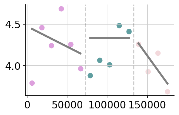
gas_obj.plot_gene_pwlinear(gene,domain_colors,offset=10**6,
                           cell_type_list=None,pt_size=50,linear_fit=True,
                           ticksize=15, figsize=(4,2.5),
                           lw=3,domain_boundary_plotting=True)

gene MARCO: discontinuous jump after domain(s) []
gene MARCO: continuous gradient in domain(s) [0, 2]

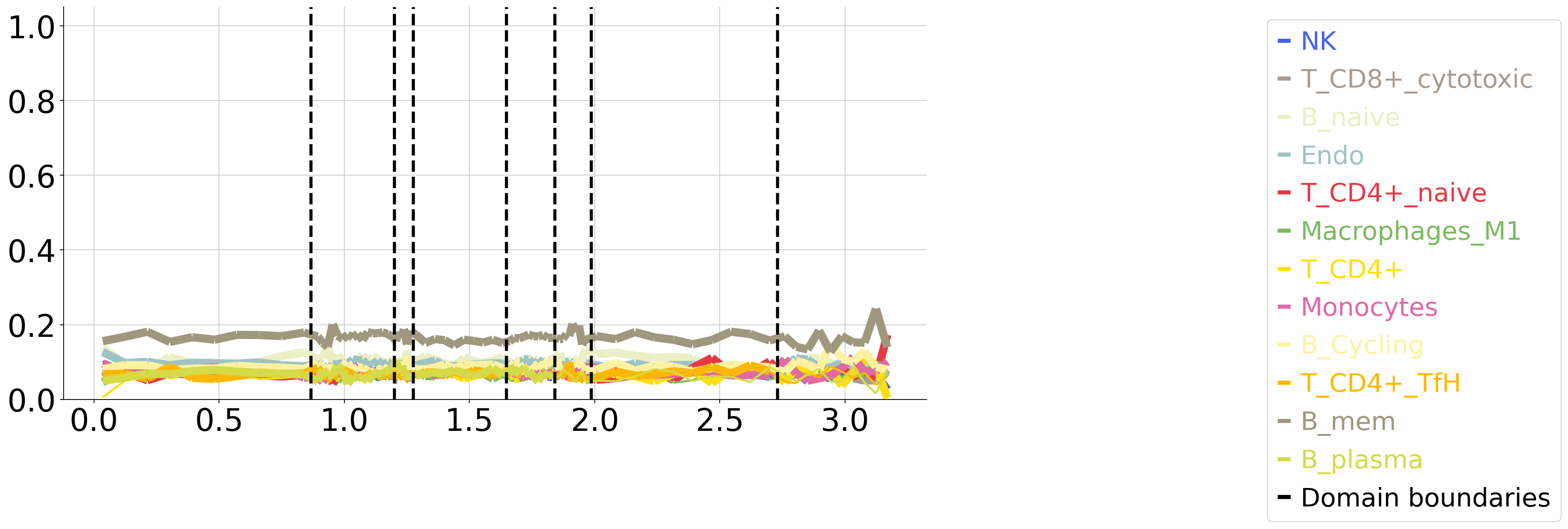
Plot cell type vs isodepth (if cell type info available)

Load cell type label per spot (from tangram). The tutorial and result could be found in https://omicverse.readthedocs.io/en/latest/Tutorials-space/t_mapping/

We store as N x C dataframe M where M[i,c]=1 if spot i is cell type c, and 0 if not

cell_type_df=ov.pd.read_csv('data/V1_Human_Lymph_Node_celltype.csv', index_col=0)
cell_type_df.head()

	Macrophages_M1	B_IFN	B_GC_LZ	Mast	B_activated	B_GC_DZ	B_mem	T_CD8+_naive	FDC	B_GC_prePB	...	Endo	T_CD8+_cytotoxic	T_CD4+	B_Cycling	T_CD4+_naive	ILC	T_CD4+_TfH	T_CD8+_CD161+	NKT	NK
AAACAAGTATCTCCCA-1	0.082171	0.000017	0.021260	0.000019	0.259048	0.030650	0.504739	0.411314	0.000519	0.000018	...	0.376284	0.043815	0.127287	0.233432	0.006444	0.064583	0.354094	0.170322	0.022457	0.199254
AAACAATCTACTAGCA-1	0.105147	0.000004	0.087364	0.000134	0.009732	0.005403	0.205373	0.039582	0.110013	0.000051	...	0.149988	0.154454	0.160099	0.229329	0.703887	0.057109	0.412450	0.003166	0.053408	0.010387
AAACACCAATAACTGC-1	0.112886	0.000004	0.023793	0.000220	0.228582	0.001881	0.536273	0.156701	0.001156	0.000022	...	0.326906	0.183677	0.110817	0.252126	0.018042	0.083709	0.134888	0.281477	0.001987	0.273480
AAACAGAGCGACTCCT-1	0.150097	0.920552	0.083713	0.089123	0.002341	0.031755	0.321248	0.003961	0.169535	0.000032	...	0.176462	0.398296	0.003631	0.270192	0.353399	0.026902	0.025387	0.015009	0.023835	0.170472
AAACAGCTTTCAGAAG-1	0.281063	0.000003	0.103263	0.000018	0.005834	0.055721	0.433569	0.025195	0.104654	0.000014	...	0.066358	0.032739	0.019467	0.076862	0.072655	0.002734	0.210401	0.037577	0.003070	0.251124

5 rows × 34 columns

from omicverse.external.gaston import plot_cell_types
ct_colors=dict(zip(
    cell_type_df.columns,
    ov.pl.sc_color+ov.utils._plot.palette_28
))
num_bins_per_domain=[10]*len(set(adata.obs['gaston_labels']))

plot_cell_types.plot_ct_props(
    cell_type_df, 
    gaston_labels, 
    gaston_isodepth, 
    num_bins_per_domain=num_bins_per_domain, 
    ct_colors=ct_colors, 
    ct_pseudocounts={3:1},
    include_lgd=True, 
    figsize=(15,7),
    ticksize=30, 
    width1=8, 
    width2=2, 
    domain_ct_threshold=0.5
)