Multi omics analysis by MOFA

MOFA is a factor analysis model that provides a general framework for the integration of multi-omic data sets in an unsupervised fashion.

This tutorial focuses on how to perform mofa in multi-omics like scRNA-seq and scATAC-seq

Paper: MOFA+: a statistical framework for comprehensive integration of multi-modal single-cell data

Code: https://github.com/bioFAM/mofapy2

Colab_Reproducibility：https://colab.research.google.com/drive/1UPGQA3BenrC-eLIGVtdKVftSnOKIwNrP?usp=sharing

Part.1 MOFA Model

In this part, we construct a model of mofa by scRNA-seq and scATAC-seq

import omicverse as ov
rna=ov.utils.read('data/sample/rna_p_n_raw.h5ad')
atac=ov.utils.read('data/sample/atac_p_n_raw.h5ad')

/Users/fernandozeng/miniforge3/envs/scbasset/lib/python3.8/site-packages/phate/__init__.py

rna,atac

(AnnData object with n_obs × n_vars = 1876 × 25596
     obs: 'Type', 'sample',
 AnnData object with n_obs × n_vars = 1876 × 71272
     obs: 'Type', 'sample')

We only need to add anndata to ov.single.mofa to construct the base model

test_mofa=ov.single.pyMOFA(omics=[rna,atac],
                             omics_name=['RNA','ATAC'])

test_mofa.mofa_preprocess()
test_mofa.mofa_run(outfile='models/brac_rna_atac.hdf5')

        #########################################################
        ###           __  __  ____  ______                    ### 
        ###          |  \/  |/ __ \|  ____/\    _             ### 
        ###          | \  / | |  | | |__ /  \ _| |_           ### 
        ###          | |\/| | |  | |  __/ /\ \_   _|          ###
        ###          | |  | | |__| | | / ____ \|_|            ###
        ###          |_|  |_|\____/|_|/_/    \_\              ###
        ###                                                   ### 
        ######################################################### 
       
 
        
Groups names not provided, using default naming convention:
- group1, group2, ..., groupG

Successfully loaded view='RNA' group='group0' with N=1876 samples and D=25596 features...
Successfully loaded view='ATAC' group='group0' with N=1876 samples and D=71272 features...


Warning: 8795 features(s) in view 0 have zero variance, consider removing them before training the model...

Warning: 34 features(s) in view 1 have zero variance, consider removing them before training the model...

Model options:
- Automatic Relevance Determination prior on the factors: True
- Automatic Relevance Determination prior on the weights: True
- Spike-and-slab prior on the factors: False
- Spike-and-slab prior on the weights: True
Likelihoods:
- View 0 (RNA): gaussian
- View 1 (ATAC): gaussian



GPU mode is activated, but GPU not found... switching to CPU mode
For GPU mode, you need:
1 - Make sure that you are running MOFA+ on a machine with an NVIDIA GPU
2 - Install CUPY following instructions on https://docs-cupy.chainer.org/en/stable/install.html



######################################
## Training the model with seed 112 ##
######################################


ELBO before training: -2415164577.49 

Iteration 1: time=55.65, ELBO=-21568895.23, deltaELBO=2393595682.263 (99.10693890%), Factors=19
Iteration 2: time=55.70, ELBO=53947093.49, deltaELBO=75515988.721 (3.12674297%), Factors=18
Iteration 3: time=55.13, ELBO=55272104.20, deltaELBO=1325010.708 (0.05486213%), Factors=17
Iteration 4: time=50.87, ELBO=55846669.26, deltaELBO=574565.064 (0.02378989%), Factors=16
Iteration 5: time=50.76, ELBO=56054695.49, deltaELBO=208026.230 (0.00861334%), Factors=16
Iteration 6: time=46.63, ELBO=56193608.97, deltaELBO=138913.480 (0.00575172%), Factors=16

Part.2 MOFA Analysis

After get the model by mofa, we need to analysis the factor about different omics, we provide some method to do this

load data

import omicverse as ov
ov.utils.ov_plot_set()

/Users/fernandozeng/miniforge3/envs/scbasset/lib/python3.8/site-packages/phate/__init__.py

rna=ov.utils.read('data/sample/rna_test.h5ad')

add value of factor to anndata

rna=ov.single.factor_exact(rna,hdf5_path='data/sample/MOFA_POS.hdf5')
rna

AnnData object with n_obs × n_vars = 1792 × 3000
    obs: 'Type', 'sample', 'cell_type', 'n_genes', 'n_genes_by_counts', 'total_counts', 'total_counts_mt', 'pct_counts_mt', 'factor1', 'factor2', 'factor3', 'factor4', 'factor5', 'factor6', 'factor7', 'factor8', 'factor9', 'factor10', 'factor11'
    var: 'n_cells', 'mt', 'n_cells_by_counts', 'mean_counts', 'pct_dropout_by_counts', 'total_counts', 'highly_variable', 'highly_variable_rank', 'means', 'variances', 'variances_norm'
    uns: 'hvg'

analysis of the correlation between factor and cell type

ov.single.factor_correlation(adata=rna,cluster='cell_type',factor_list=[1,2,3,4,5])

	factor1	factor2	factor3	factor4	factor5
B cell-2	9.078459	5.625337	8.424565	7.768767	0.268084
B cell-1	0.489567	3.898347	0.115866	0.854649	0.686837
B cell-4	0.279002	3.701674	0.487245	0.631280	0.205712
Natural killer cell	1.127901	27.896554	0.235219	0.241705	0.282893
B cell-3	0.706249	40.881023	2.267589	0.382177	5.123728
T cell-1	0.704842	3.701813	0.464042	0.396243	0.459828
Endothelial cell	NaN	NaN	NaN	NaN	NaN
Monocyte	0.248902	0.284968	0.147168	0.399443	0.132685
Epithelial cell	0.435818	2.957245	0.183706	0.366285	0.225828
Natural killer T (NKT) cell-1	0.119266	0.276104	0.111210	0.030626	0.097991
Plasmacytoid dendritic cell	0.019003	0.052997	0.431551	0.024616	0.067029
Regulatory T (Treg) cell	0.553421	7.303644	0.323052	0.252761	0.187171
B cell	1.096582	12.407881	0.154599	0.827906	0.495789
Natural killer T (NKT) cell	0.039153	0.765500	0.243345	0.035279	0.093851
T cell	1.763401	32.202576	0.854274	0.870854	0.627218

Get the gene/feature weights of different factor

ov.single.get_weights(hdf5_path='data/sample/MOFA_POS.hdf5',view='RNA',factor=1)

	feature	weights	abs_weights	sig
0	b'FAM174B'	-2.911107e-10	2.911107e-10	-
1	b'SYNE2'	-3.744153e-09	3.744153e-09	-
2	b'LUZP1'	-1.840838e-10	1.840838e-10	-
3	b'GGT1'	-3.171818e-10	3.171818e-10	-
4	b'LINC02210'	-4.588388e-10	4.588388e-10	-
...	...	...	...	...
2995	b'TREM2'	4.046089e-11	4.046089e-11	+
2996	b'CPVL'	1.353563e-10	1.353563e-10	+
2997	b'MIPEP'	-1.360450e-11	1.360450e-11	-
2998	b'INO80E'	-4.721143e-09	4.721143e-09	-
2999	b'RABAC1'	2.386149e-03	2.386149e-03	+

3000 rows × 4 columns

Part.3 MOFA Visualize

To visualize the result of mofa, we provide a series of function to do this.

pymofa_obj=ov.single.pyMOFAART(model_path='data/sample/MOFA_POS.hdf5')

We get the factor of each cell at first

pymofa_obj.get_factors(rna)
rna

......Add factors to adata and store to adata.obsm["X_mofa"]

AnnData object with n_obs × n_vars = 1792 × 3000
    obs: 'Type', 'sample', 'cell_type', 'n_genes', 'n_genes_by_counts', 'total_counts', 'total_counts_mt', 'pct_counts_mt', 'factor1', 'factor2', 'factor3', 'factor4', 'factor5', 'factor6', 'factor7', 'factor8', 'factor9', 'factor10', 'factor11'
    var: 'n_cells', 'mt', 'n_cells_by_counts', 'mean_counts', 'pct_dropout_by_counts', 'total_counts', 'highly_variable', 'highly_variable_rank', 'means', 'variances', 'variances_norm'
    uns: 'hvg'
    obsm: 'X_mofa'

We can also plot the varience in each View

pymofa_obj.plot_r2()

(<Figure size 160x240 with 2 Axes>,
 <Axes: title={'center': 'Varience'}, xlabel='View', ylabel='Factor'>)

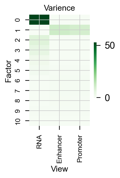
pymofa_obj.get_r2()

	RNA	Enhancer	Promoter
0	52.653359	0.020433	0.030287
1	-0.427822	11.423973	10.044684
2	7.485323	0.042972	0.044618
3	5.582933	0.029609	0.040193
4	2.447518	0.084279	0.102553
5	1.264806	0.379936	0.315503
6	0.142767	0.743871	0.637848
7	0.066169	0.717554	0.653633
8	0.061457	0.451830	0.363793
9	0.322288	0.275757	0.240563
10	0.132726	0.044343	0.059752

Visualize the correlation between factor and celltype

pymofa_obj.plot_cor(rna,'cell_type')

(<Figure size 480x240 with 2 Axes>,
 <Axes: title={'center': 'Correlation'}, xlabel='Factor', ylabel='cell_type'>)

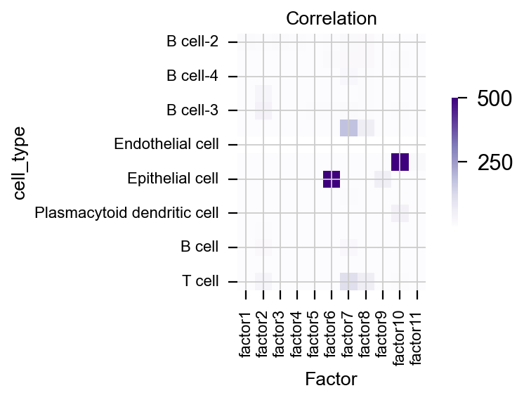
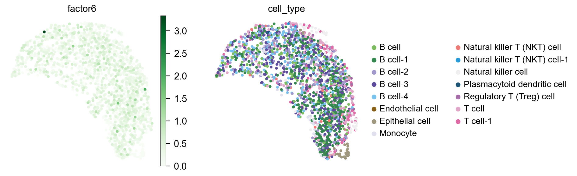
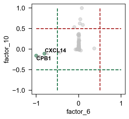
We found that factor6 is correlated to Epithelial

pymofa_obj.plot_factor(rna,'cell_type','Epi',figsize=(3,3),
                    factor1=6,factor2=10,)

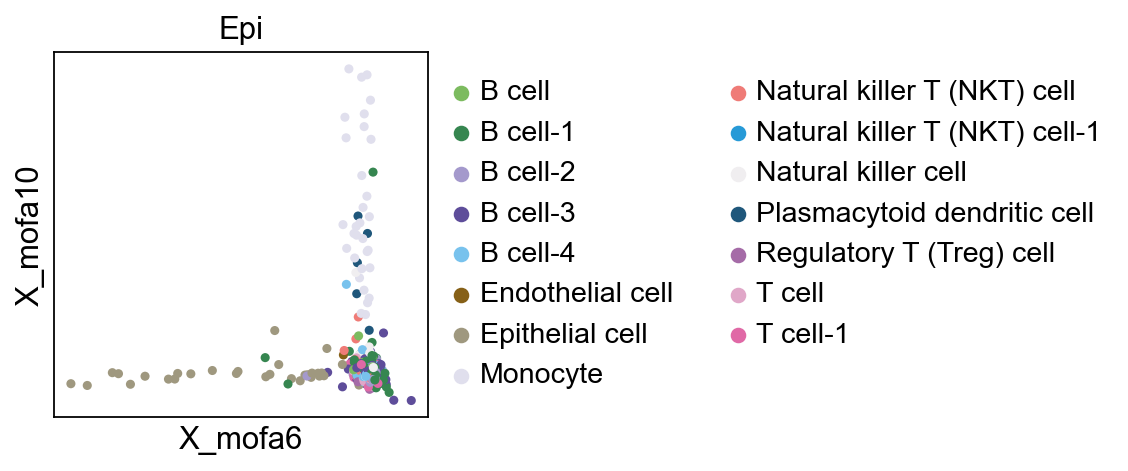
(<Figure size 240x240 with 1 Axes>,
 <Axes: title={'center': 'Epi'}, xlabel='X_mofa6', ylabel='X_mofa10'>)

import scanpy as sc
sc.pp.neighbors(rna)
sc.tl.umap(rna)
sc.pl.embedding(
    rna,
    basis="X_umap",
    color=["factor6","cell_type"],
    frameon=False,
    ncols=2,
    #palette=ov.utils.pyomic_palette(),
    show=False,
    cmap='Greens',
    vmin=0,
)
#plt.savefig("figures/umap_factor6.png",dpi=300,bbox_inches = 'tight')

computing neighbors
    using 'X_pca' with n_pcs = 50
    finished: added to `.uns['neighbors']`
    `.obsp['distances']`, distances for each pair of neighbors
    `.obsp['connectivities']`, weighted adjacency matrix (0:00:00)
computing UMAP
    finished: added
    'X_umap', UMAP coordinates (adata.obsm) (0:00:01)

[<Axes: title={'center': 'factor6'}, xlabel='X_umap1', ylabel='X_umap2'>,
 <Axes: title={'center': 'cell_type'}, xlabel='X_umap1', ylabel='X_umap2'>]

pymofa_obj.plot_weight_gene_d1(view='RNA',factor1=6,factor2=10,)

(<Figure size 240x240 with 1 Axes>,
 <Axes: xlabel='factor_6', ylabel='factor_10'>)

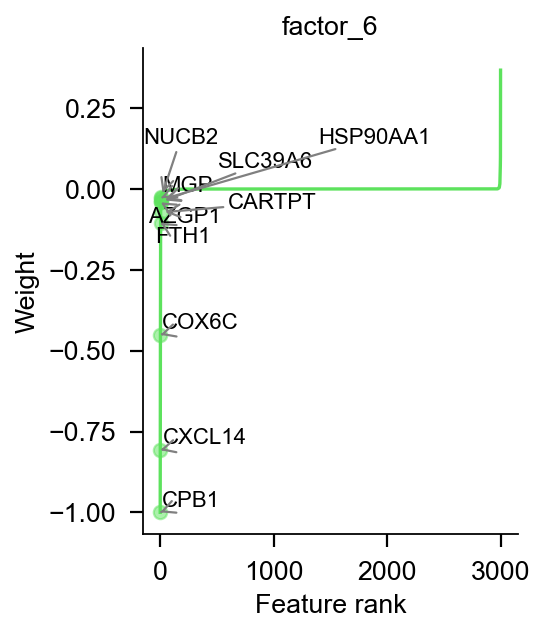
pymofa_obj.plot_weights(view='RNA',factor=6,color='#5de25d',
                        ascending=True)

(<Figure size 240x320 with 1 Axes>,
 <Axes: title={'center': 'factor_6'}, xlabel='Feature rank', ylabel='Weight'>)

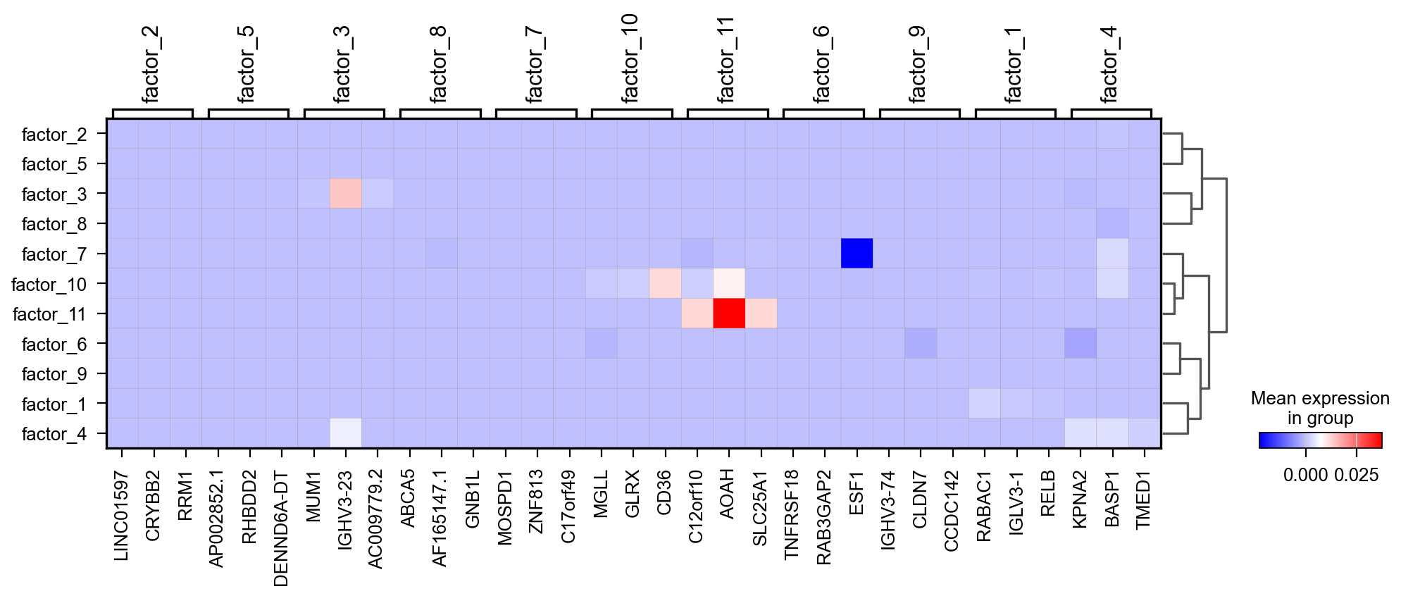
pymofa_obj.plot_top_feature_heatmap(view='RNA')

ranking genes
    finished: added to `.uns['rank_genes_groups']`
    'names', sorted np.recarray to be indexed by group ids
    'scores', sorted np.recarray to be indexed by group ids
    'logfoldchanges', sorted np.recarray to be indexed by group ids
    'pvals', sorted np.recarray to be indexed by group ids
    'pvals_adj', sorted np.recarray to be indexed by group ids (0:00:00)
WARNING: dendrogram data not found (using key=dendrogram_Factor). Running `sc.tl.dendrogram` with default parameters. For fine tuning it is recommended to run `sc.tl.dendrogram` independently.
WARNING: You’re trying to run this on 3000 dimensions of `.X`, if you really want this, set `use_rep='X'`.
         Falling back to preprocessing with `sc.pp.pca` and default params.
computing PCA
    with n_comps=21
    finished (0:00:00)
Storing dendrogram info using `.uns['dendrogram_Factor']`

{'mainplot_ax': <Axes: >,
 'group_extra_ax': <Axes: >,
 'gene_group_ax': <Axes: >,
 'color_legend_ax': <Axes: title={'center': 'Mean expression\nin group'}>}