Bulk RNA-seq generate ‘interrupted’ cells to interpolate scRNA-seq

The limited number of cells available for single-cell sequencing has led to ‘interruptions’ in the study of cell development and differentiation trajectories. In contrast, bulk RNA-seq sequencing of whole tissues contains, in principle, ‘interrupted’ cells. To our knowledge, there is no algorithm for extracting ‘interrupted’ cells from bulk RNA-seq. There is a lack of tools that effectively bridge the gap between bulk-seq and single-seq analyses.

We developed BulkTrajBlend in OmicVerse, which is specifically designed to address cell continuity in single-cell sequencing.BulkTrajBlend first deconvolves single-cell data from Bulk RNA-seq and then uses a GNN-based overlapping community discovery algorithm to identify contiguous cells in the generated single-cell data.

Colab_Reproducibility：https://colab.research.google.com/drive/1HulVXQIlUEcpGRDZo4MxcHYOjnVhuCC-?usp=sharing

import omicverse as ov
from omicverse.utils import mde
import scanpy as sc
import scvelo as scv
ov.plot_set()

   ____            _     _    __                  
  / __ \____ ___  (_)___| |  / /__  _____________ 
 / / / / __ `__ \/ / ___/ | / / _ \/ ___/ ___/ _ \ 
/ /_/ / / / / / / / /__ | |/ /  __/ /  (__  )  __/ 
\____/_/ /_/ /_/_/\___/ |___/\___/_/  /____/\___/                                              

Version: 1.5.6, Tutorials: https://omicverse.readthedocs.io/

loading data

For illustration, we apply differential kinetic analysis to dentate gyrus neurogenesis, which comprises multiple heterogeneous subpopulations.

We utilized single-cell RNA-seq data (GEO accession: GSE95753) obtained from the dentate gyrus of the hippocampus in rats, along with bulk RNA-seq data (GEO accession: GSE74985).

adata=scv.datasets.dentategyrus()
adata

AnnData object with n_obs × n_vars = 2930 × 13913
    obs: 'clusters', 'age(days)', 'clusters_enlarged'
    uns: 'clusters_colors'
    obsm: 'X_umap'
    layers: 'ambiguous', 'spliced', 'unspliced'

import numpy as np
bulk=ov.utils.read('data/GSE74985_mergedCount.txt.gz',index_col=0)
bulk=ov.bulk.Matrix_ID_mapping(bulk,'genesets/pair_GRCm39.tsv')
bulk.head()

	dg_d_1	dg_d_2	dg_d_3	dg_v_1	dg_v_2	dg_v_3	ca4_1	ca4_2	ca4_3	ca3_d_1	...	ca3_v_3	ca2_1	ca2_2	ca2_3	ca1_d_1	ca1_d_2	ca1_d_3	ca1_v_1	ca1_v_2	ca1_v_3
Adat1	70	46	49	150	150	99	164	33	29	76	...	64	87	86	21	42	143	23	26	10	23
Gm12094	0	103	0	21	5	2	0	5	0	0	...	0	10	0	0	1	0	1	0	0	0
Olfr203	0	0	0	0	0	0	0	0	0	0	...	0	0	0	0	0	0	0	0	0	0
Mageb5b	0	0	0	0	0	0	0	0	0	0	...	0	0	0	0	0	0	0	0	0	0
Top2a	0	0	5	0	19	0	0	18	1	0	...	0	37	0	2	0	0	0	0	0	0

5 rows × 24 columns

Configure the BulkTrajBlend model

Here, we import the bulk RNA-seq and scRNA-seq data we have just prepared as input into the BulkTrajBlend model. We use the lazy function for preprocessing and we note that dg_d represents the neuronal data of the dentate gyrus, which we merge as it is three replicates.

Note that the bulk RNA-seq and scRNA-seq we use here are raw data, not normalised and logarithmic, and are not suitable for use with the lazy function if your data has already been processed. It is important to note that single cell data cannot be scale

cell_target_num represents the expected number of cells in each category and we do not use a least squares approach to fit the cell proportions here. If we set None, We use TAPE by default to estimate the proportion of each type of cell, but of course you can also specify the number of cells directly

bulktb=ov.bulk2single.BulkTrajBlend(bulk_seq=bulk,single_seq=adata,
                                    bulk_group=['dg_d_1','dg_d_2','dg_d_3'],
                                    celltype_key='clusters',)

bulktb.vae_configure(cell_target_num=100)

......drop duplicates index in bulk data
......deseq2 normalize the bulk data
......log10 the bulk data
......calculate the mean of each group
......normalize the single data
normalizing counts per cell
    finished (0:00:00)
......log1p the single data
......prepare the input of bulk2single
...loading data

Training the beta-VAE model

We first generated single cell data from the bulk RNA-seq data using beta-VAE and filtered out noisy cells using the size of the leiden as a constraint.

cell_target_num represents the expected number of cells in each category and we do not use a least squares approach to fit the cell proportions here.

vae_net=bulktb.vae_train(
    batch_size=512,
    learning_rate=1e-4,
    hidden_size=256,
    epoch_num=3500,
    vae_save_dir='data/bulk2single/save_model',
    vae_save_name='dg_btb_vae',
    generate_save_dir='data/bulk2single/output',
    generate_save_name='dg_btb')

...begin vae training
min loss = 0.8291964083909988
...vae training done!
...save trained vae in data/bulk2single/save_model/dg_btb_vae.pth.

bulktb.vae_load('data/bulk2single/save_model/dg_btb_vae.pth')

loading model from data/bulk2single/save_model/dg_btb_vae.pth
loading model from data/bulk2single/save_model/dg_btb_vae.pth

generate_adata=bulktb.vae_generate(leiden_size=25)

...generating
generated done!
extracting highly variable genes
    finished (0:00:00)
--> added
    'highly_variable', boolean vector (adata.var)
    'means', float vector (adata.var)
    'dispersions', float vector (adata.var)
    'dispersions_norm', float vector (adata.var)
computing PCA
Note that scikit-learn's randomized PCA might not be exactly reproducible across different computational platforms. For exact reproducibility, choose `svd_solver='arpack'.`
    on highly variable genes
    with n_comps=100
    finished (0:00:00)
computing neighbors
    finished: added to `.uns['neighbors']`
    `.obsp['distances']`, distances for each pair of neighbors
    `.obsp['connectivities']`, weighted adjacency matrix (0:00:01)
running Leiden clustering
    finished: found 28 clusters and added
    'leiden', the cluster labels (adata.obs, categorical) (0:00:00)
The filter leiden is  ['14', '15', '16', '17', '18', '19', '20', '21', '22', '23', '24', '25', '26', '27']

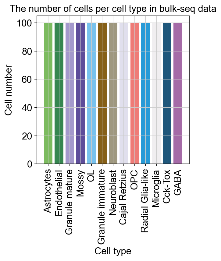
ov.bulk2single.bulk2single_plot_cellprop(generate_adata,celltype_key='clusters',
                                        )

<AxesSubplot: title={'center': 'The number of cells per cell type in bulk-seq data'}, xlabel='Cell type', ylabel='Cell number'>

Visualize the generate scRNA-seq

To visualize the generate scRNA-seq’s learned embeddings, we use the pymde package wrapperin omicverse. This is an alternative to UMAP that is GPU-accelerated.

Training the GNN model

Next, we used GNN to look for overlapping communities (community = cell type) in the generated single-cell data.

• gpu: The GPU ID for training the GNN model. Default is 0.

• hidden_size: The hidden size for the GNN model. Default is 128.

• weight_decay: The weight decay for the GNN model. Default is 1e-2.

• dropout: The dropout for the GNN model. Default is 0.5.

• batch_norm: Whether to use batch normalization for the GNN model. Default is True.

• lr: The learning rate for the GNN model. Default is 1e-3.

• max_epochs: The maximum epoch number for training the GNN model. Default is 500.

• display_step: The display step for training the GNN model. Default is 25.

• balance_loss: Whether to use the balance loss for training the GNN model. Default is True.

• stochastic_loss: Whether to use the stochastic loss for training the GNN model. Default is True.

• batch_size: The batch size for training the GNN model. Default is 2000.

• num_workers: The number of workers for training the GNN model. Default is 5.

bulktb.gnn_configure(max_epochs=2000,use_rep='X',
                     neighbor_rep='X_pca')

torch have been install version: 2.0.1
computing neighbors
    finished: added to `.uns['neighbors']`
    `.obsp['distances']`, distances for each pair of neighbors
    `.obsp['connectivities']`, weighted adjacency matrix (0:00:00)

There are many parameters that can be controlled during training, here we set them all to the default

• thresh: the threshold for filtered the overlap community

• gnn_save_dir: the save dir for gnn model

• gnn_save_name: the gnn model name to save

bulktb.gnn_train()

Breaking due to early stopping at epoch 850
......add nocd result to adata.obs
...save trained gnn in save_model/gnn.pth.

Since the previously generated single cell data has a random nature in the construction of the neighbourhood map, the model must be loaded on the fixed generated single cell data. Otherwise an error will be reported

bulktb.gnn_load('save_model/gnn.pth')

We can use GNN to get an overlapping community for each cell.

res_pd=bulktb.gnn_generate()
res_pd.head()

The nocd result is  nocd_Cck-Tox             157
nocd_Microglia           100
nocd_OPC                 158
nocd_Astrocytes          198
nocd_Mossy                81
nocd_OL                   98
nocd_Cajal Retzius       119
nocd_Endothelial_1        54
nocd_Granule immature    150
nocd_Neuroblast          104
nocd_Cck-Tox_1            74
nocd_Endothelial          72
nocd_GABA                101
dtype: int64
The nocd result has been added to adata.obs['nocd_']

	nocd_Cck-Tox	nocd_Microglia	nocd_OPC	nocd_Astrocytes	nocd_Mossy	nocd_OL	nocd_Cajal Retzius	nocd_Endothelial_1	nocd_Granule immature	nocd_Neuroblast	nocd_Cck-Tox_1	nocd_Endothelial	nocd_GABA
C_1	0	0	0	1	0	0	0	0	0	0	0	0	0
C_2	0	0	0	1	0	0	0	0	0	0	0	0	0
C_3	0	0	0	0	0	0	0	0	0	0	0	1	0
C_4	1	0	0	0	0	0	0	0	1	0	0	0	0
C_5	0	0	0	0	1	0	0	0	0	0	0	0	0

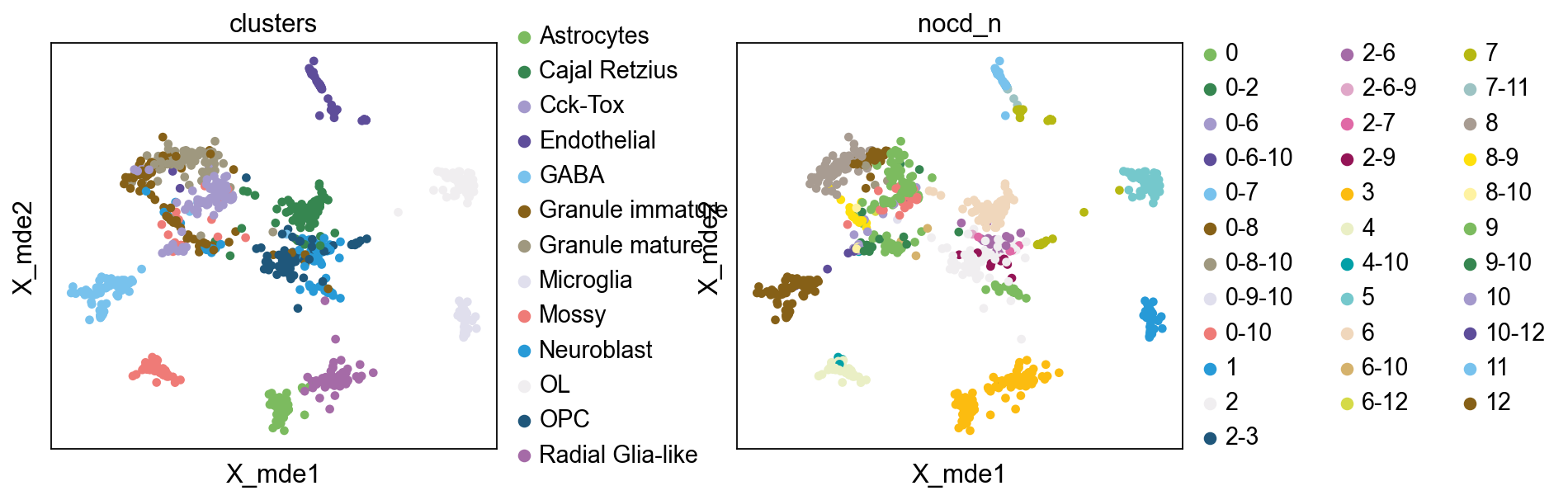
bulktb.nocd_obj.adata.obsm["X_mde"] = mde(bulktb.nocd_obj.adata.obsm["X_pca"])
sc.pl.embedding(bulktb.nocd_obj.adata,basis='X_mde',color=['clusters','nocd_n'],wspace=0.4,
          palette=ov.utils.pyomic_palette())

WARNING: Length of palette colors is smaller than the number of categories (palette length: 28, categories length: 34. Some categories will have the same color.

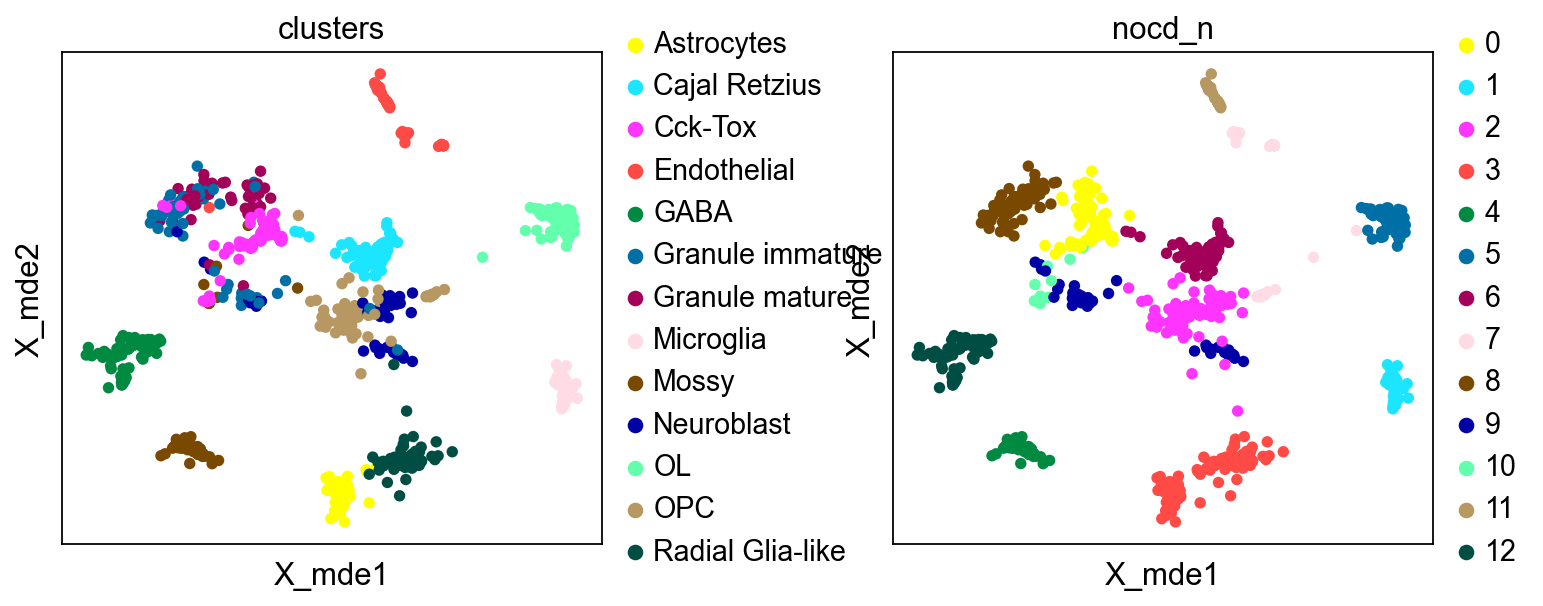
sc.pl.embedding(bulktb.nocd_obj.adata[~bulktb.nocd_obj.adata.obs['nocd_n'].str.contains('-')],
                basis='X_mde',
           color=['clusters','nocd_n'],
           wspace=0.4,palette=sc.pl.palettes.default_102)

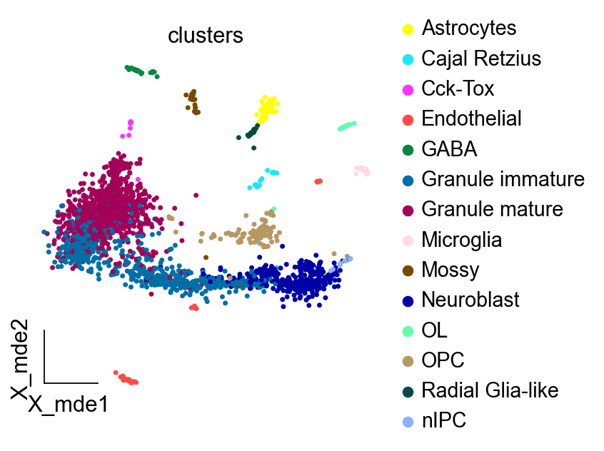
Interpolation of the “interruption” cell

A simple function is provided to interpolate the “interruption” cells in the original data, making the single cell data continuous.

print('raw cells: ',bulktb.single_seq.shape[0])
#adata1=bulktb.interpolation('Neuroblast')
adata1=bulktb.interpolation('OPC')
print('interpolation cells: ',adata1.shape[0])

raw cells:  2930
interpolation cells:  3088

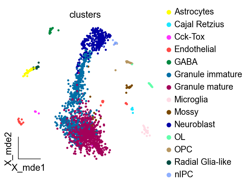
Visualisation of single cell data before and after interpolation

adata1.raw = adata1
sc.pp.highly_variable_genes(adata1, min_mean=0.0125, max_mean=3, min_disp=0.5)
adata1 = adata1[:, adata1.var.highly_variable]
sc.pp.scale(adata1, max_value=10)

extracting highly variable genes
    finished (0:00:00)
--> added
    'highly_variable', boolean vector (adata.var)
    'means', float vector (adata.var)
    'dispersions', float vector (adata.var)
    'dispersions_norm', float vector (adata.var)
... as `zero_center=True`, sparse input is densified and may lead to large memory consumption

sc.tl.pca(adata1, n_comps=100, svd_solver="auto")

computing PCA
Note that scikit-learn's randomized PCA might not be exactly reproducible across different computational platforms. For exact reproducibility, choose `svd_solver='arpack'.`
    on highly variable genes
    with n_comps=100
    finished (0:00:00)

sc.pp.normalize_total(adata, target_sum=1e4)
sc.pp.log1p(adata)
adata.raw = adata
sc.pp.highly_variable_genes(adata, min_mean=0.0125, max_mean=3, min_disp=0.5)
adata = adata[:, adata.var.highly_variable]
sc.pp.scale(adata, max_value=10)

normalizing counts per cell
    finished (0:00:00)
extracting highly variable genes
    finished (0:00:00)
--> added
    'highly_variable', boolean vector (adata.var)
    'means', float vector (adata.var)
    'dispersions', float vector (adata.var)
    'dispersions_norm', float vector (adata.var)
... as `zero_center=True`, sparse input is densified and may lead to large memory consumption

sc.tl.pca(adata, n_comps=100, svd_solver="auto")

computing PCA
Note that scikit-learn's randomized PCA might not be exactly reproducible across different computational platforms. For exact reproducibility, choose `svd_solver='arpack'.`
    on highly variable genes
    with n_comps=100
    finished (0:00:00)

adata.obsm["X_mde"] = mde(adata.obsm["X_pca"])
adata1.obsm["X_mde"] = mde(adata1.obsm["X_pca"])

ov.utils.embedding(adata,
                basis='X_mde',
           color=['clusters'],
                   frameon='small',
           wspace=0.4,palette=sc.pl.palettes.default_102)

ov.utils.embedding(adata1,
                basis='X_mde',
           color=['clusters'],
                frameon='small',
           wspace=0.4,palette=sc.pl.palettes.default_102)

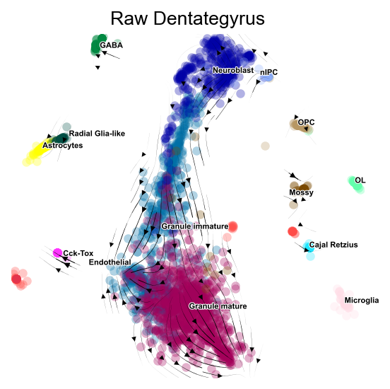
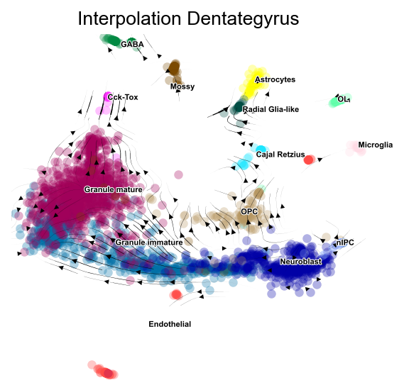
Visualisation of the proposed time series trajectory of cells before and after interpolation

Here, we use pyVIA to complete the calculation of the pseudotime .

v0 = ov.single.pyVIA(adata=adata,adata_key='X_pca',adata_ncomps=100, basis='X_mde',
                         clusters='clusters',knn=20,random_seed=4,root_user=['nIPC'],
                    dataset='group')
v0.run()

v1 = ov.single.pyVIA(adata=adata1,adata_key='X_pca',adata_ncomps=100, basis='X_mde',
                         clusters='clusters',knn=15,random_seed=4,root_user=['Neuroblast'],
                     #jac_std_global=0.01,
                    dataset='group')

v1.run()

import matplotlib.pyplot as plt
fig,ax=v0.plot_stream(basis='X_mde',clusters='clusters',
               density_grid=0.8, scatter_size=30, scatter_alpha=0.3, linewidth=0.5)
plt.title('Raw Dentategyrus',fontsize=12)
#fig.savefig('figures/v0_via_fig4.png',dpi=300,bbox_inches = 'tight')

Text(0.5, 1.0, 'Raw Dentategyrus')

fig,ax=v1.plot_stream(basis='X_mde',clusters='clusters',
               density_grid=0.8, scatter_size=30, scatter_alpha=0.3, linewidth=0.5)
plt.title('Interpolation Dentategyrus',fontsize=12)
#fig.savefig('figures/v1_via_fig4.png',dpi=300,bbox_inches = 'tight')

Text(0.5, 1.0, 'Interpolation Dentategyrus')

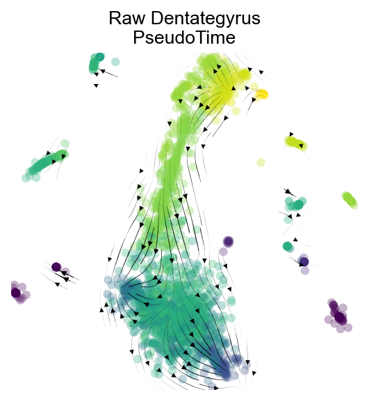
fig,ax=v0.plot_stream(basis='X_mde',density_grid=0.8, scatter_size=30, color_scheme='time', linewidth=0.5,
                             min_mass = 1, cutoff_perc = 5, scatter_alpha=0.3, marker_edgewidth=0.1,
                             density_stream = 2, smooth_transition=1, smooth_grid=0.5)
plt.title('Raw Dentategyrus\nPseudoTime',fontsize=12)

Text(0.5, 1.0, 'Raw Dentategyrus\nPseudoTime')

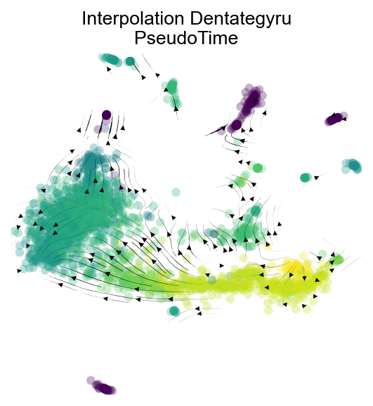
fig,ax=v1.plot_stream(basis='X_mde',density_grid=0.8, scatter_size=30, color_scheme='time', linewidth=0.5,
                             min_mass = 1, cutoff_perc = 5, scatter_alpha=0.3, marker_edgewidth=0.1,
                             density_stream = 2, smooth_transition=1, smooth_grid=0.5)
plt.title('Interpolation Dentategyru\nPseudoTime',fontsize=12)

Text(0.5, 1.0, 'Interpolation Dentategyru\nPseudoTime')

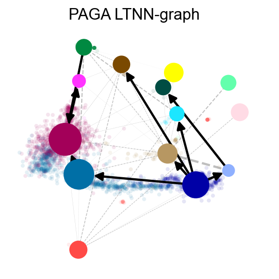
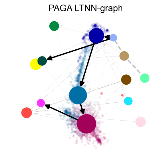
PAGA Graph

To visualize the state transfer matrix, here we use PAGA to compute the state transfer diagram to further verify that our differentiation trajectory is valid

v0.get_pseudotime(adata)
sc.pp.neighbors(adata,n_neighbors= 15,use_rep='X_pca')
ov.utils.cal_paga(adata,use_time_prior='pt_via',vkey='paga',
                 groups='clusters')

...the pseudotime of VIA added to AnnData obs named `pt_via`
computing neighbors
    finished: added to `.uns['neighbors']`
    `.obsp['distances']`, distances for each pair of neighbors
    `.obsp['connectivities']`, weighted adjacency matrix (0:00:00)
running PAGA using priors: ['pt_via']
    finished
added
    'paga/connectivities', connectivities adjacency (adata.uns)
    'paga/connectivities_tree', connectivities subtree (adata.uns)
    'paga/transitions_confidence', velocity transitions (adata.uns)

ov.utils.plot_paga(adata,basis='mde', size=50, alpha=.1,title='PAGA LTNN-graph',
            min_edge_width=2, node_size_scale=1.5,show=False,legend_loc=False)

<AxesSubplot: title={'center': 'PAGA LTNN-graph'}>

v1.get_pseudotime(adata1)
sc.pp.neighbors(adata1,n_neighbors= 15,use_rep='X_pca')
ov.utils.cal_paga(adata1,use_time_prior='pt_via',vkey='paga',
                 groups='clusters')

...the pseudotime of VIA added to AnnData obs named `pt_via`
computing neighbors
    finished: added to `.uns['neighbors']`
    `.obsp['distances']`, distances for each pair of neighbors
    `.obsp['connectivities']`, weighted adjacency matrix (0:00:00)
running PAGA using priors: ['pt_via']
    finished
added
    'paga/connectivities', connectivities adjacency (adata.uns)
    'paga/connectivities_tree', connectivities subtree (adata.uns)
    'paga/transitions_confidence', velocity transitions (adata.uns)

ov.utils.plot_paga(adata1,basis='mde', size=50, alpha=.1,title='PAGA LTNN-graph',
            min_edge_width=2, node_size_scale=1.5,show=False,legend_loc=False)

<AxesSubplot: title={'center': 'PAGA LTNN-graph'}>