GeneModule Identified

In omicverse, we prepared two methods to identify the gene module, one is cNMF, the other one is hospot.

import scanpy as sc
import omicverse as ov
ov.style(font_path='Arial')

%load_ext autoreload
%autoreload 2

🔬 Starting plot initialization...
Using already downloaded Arial font from: /tmp/omicverse_arial.ttf
Registered as: Arial
🧬 Detecting GPU devices…
✅ NVIDIA CUDA GPUs detected: 1
    • [CUDA 0] NVIDIA H100 80GB HBM3
      Memory: 79.1 GB | Compute: 9.0

   ____            _     _    __                  
  / __ \____ ___  (_)___| |  / /__  _____________ 
 / / / / __ `__ \/ / ___/ | / / _ \/ ___/ ___/ _ \ 
/ /_/ / / / / / / / /__ | |/ /  __/ /  (__  )  __/ 
\____/_/ /_/ /_/_/\___/ |___/\___/_/  /____/\___/                                              

🔖 Version: 1.7.9rc1   📚 Tutorials: https://omicverse.readthedocs.io/
✅ plot_set complete.

Loading dataset

Here, we use the dentategyrus dataset as an example for cNMF or Hospot.

adata=ov.datasets.pancreatic_endocrinogenesis()

🔍 Downloading data to ./data/endocrinogenesis_day15.h5ad
⚠️ File ./data/endocrinogenesis_day15.h5ad already exists
 Loading data from ./data/endocrinogenesis_day15.h5ad
✅ Successfully loaded: 3696 cells × 27998 genes

%%time
adata=ov.pp.preprocess(adata,mode='shiftlog|pearson',n_HVGs=2000,)
adata

🔍 [2026-01-07 17:06:35] Running preprocessing in 'cpu' mode...
Begin robust gene identification
    After filtration, 17750/27998 genes are kept.
    Among 17750 genes, 16426 genes are robust.
✅ Robust gene identification completed successfully.
Begin size normalization: shiftlog and HVGs selection pearson

🔍 Count Normalization:
   Target sum: 500000.0
   Exclude highly expressed: True
   Max fraction threshold: 0.2
   ⚠️ Excluding 1 highly-expressed genes from normalization computation
   Excluded genes: ['Ghrl']

✅ Count Normalization Completed Successfully!
   ✓ Processed: 3,696 cells × 16,426 genes
   ✓ Runtime: 0.25s

🔍 Highly Variable Genes Selection (Experimental):
   Method: pearson_residuals
   Target genes: 2,000
   Theta (overdispersion): 100

✅ Experimental HVG Selection Completed Successfully!
   ✓ Selected: 2,000 highly variable genes out of 16,426 total (12.2%)
   ✓ Results added to AnnData object:
     • 'highly_variable': Boolean vector (adata.var)
     • 'highly_variable_rank': Float vector (adata.var)
     • 'highly_variable_nbatches': Int vector (adata.var)
     • 'highly_variable_intersection': Boolean vector (adata.var)
     • 'means': Float vector (adata.var)
     • 'variances': Float vector (adata.var)
     • 'residual_variances': Float vector (adata.var)
    Time to analyze data in cpu: 1.11 seconds.
✅ Preprocessing completed successfully.
    Added:
        'highly_variable_features', boolean vector (adata.var)
        'means', float vector (adata.var)
        'variances', float vector (adata.var)
        'residual_variances', float vector (adata.var)
        'counts', raw counts layer (adata.layers)
    End of size normalization: shiftlog and HVGs selection pearson
CPU times: user 1.43 s, sys: 717 ms, total: 2.15 s
Wall time: 1.51 s

AnnData object with n_obs × n_vars = 3696 × 16426
    obs: 'clusters_coarse', 'clusters', 'S_score', 'G2M_score'
    var: 'highly_variable_genes', 'n_cells', 'percent_cells', 'robust', 'highly_variable_features', 'means', 'variances', 'residual_variances', 'highly_variable_rank', 'highly_variable'
    uns: 'clusters_coarse_colors', 'clusters_colors', 'day_colors', 'neighbors', 'pca', 'log1p', 'hvg', 'status', 'status_args', 'REFERENCE_MANU'
    obsm: 'X_pca', 'X_umap'
    layers: 'spliced', 'unspliced', 'counts'
    obsp: 'distances', 'connectivities'

ov.pp.scale(adata)
ov.pp.pca(adata)

computing PCA🔍
    with n_comps=50
   🖥️ Using sklearn PCA for CPU computation
   🖥️ sklearn PCA backend: CPU computation
    finished✅ (0:00:02)

import matplotlib.pyplot as plt
from matplotlib import patheffects
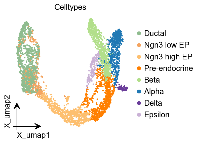
fig, ax = plt.subplots(figsize=(4,4))
ov.pl.embedding(
    adata,
    basis="X_umap",
    color=['clusters'],
    frameon='small',
    title="Celltypes",
    #legend_loc='on data',
    legend_fontsize=14,
    legend_fontoutline=2,
    #size=10,
    ax=ax,
    #legend_loc=True, 
    add_outline=False, 
    #add_outline=True,
    outline_color='black',
    outline_width=1,
    show=False,
)

<Axes: title={'center': 'Celltypes'}, xlabel='X_umap1', ylabel='X_umap2'>

Consensus Non-negative Matrix factorization (cNMF)

cNMF is an analysis pipeline for inferring gene expression programs from single-cell RNA-Seq (scRNA-Seq) data.

It takes a count matrix (N cells X G genes) as input and produces a (K x G) matrix of gene expression programs (GEPs) and a (N x K) matrix specifying the usage of each program for each cell in the data. You can read more about the method in the github and check out examples on dentategyrus.

• Dylan KotliarAdrian VeresM Aurel NagyShervin TabriziEran HodisDouglas A MeltonPardis C Sabeti (2019) Identifying gene expression programs of cell-type identity and cellular activity with single-cell RNA-Seq eLife 8:e43803.

Initialize and Training model

In omicverse, you can set use_gpu=True to perform the NMF analysis using torchnmf package, it’s easy to install using pip install torchnmf. But it should be noticed the accurancy is different if you use use_gpu=True mode.

import numpy as np
## Initialize the cnmf object that will be used to run analyses
cnmf_obj = ov.single.cNMF(
    adata,components=np.arange(5,15), n_iter=20, 
    seed=14, num_highvar_genes=2000,
    output_dir=None, name='pancrea_cNMF',use_gpu=True
)

normalizing counts per cell
    finished (0:00:00)

## Specify that the jobs are being distributed over a single worker (total_workers=1) and then launch that worker
cnmf_obj.factorize(worker_i=0, total_workers=1)

🚀 Running NMF on GPU (device 0)
Running 200 factorization iterations for worker 0...
✓ Worker 0 completed 200 iterations. Total in memory: 200

if u want to accerlate the calculation, you can try the code below

#cnmf_obj.factorize(worker_i=0, total_workers=2)
#cnmf_obj.factorize(worker_i=1, total_workers=2)

cnmf_obj.combine(skip_missing_files=True)

Combining factorizations for k=5.
  Found all 20 iterations for k=5
Combining factorizations for k=6.
  Found all 20 iterations for k=6
Combining factorizations for k=7.
  Found all 20 iterations for k=7
Combining factorizations for k=8.
  Found all 20 iterations for k=8
Combining factorizations for k=9.
  Found all 20 iterations for k=9
Combining factorizations for k=10.
  Found all 20 iterations for k=10
Combining factorizations for k=11.
  Found all 20 iterations for k=11
Combining factorizations for k=12.
  Found all 20 iterations for k=12
Combining factorizations for k=13.
  Found all 20 iterations for k=13
Combining factorizations for k=14.
  Found all 20 iterations for k=14

cnmf_obj.save('test/cnmf_obj.pkl')

✓ cNMF object saved to: test/cnmf_obj.pkl
  - 200 factorization iterations
  - 10 merged spectra (K values)
  - 0 consensus results

cnmf_obj.load('test/cnmf_obj.pkl')

📂 Load Operation:
   Source path: test/cnmf_obj.pkl
   Using: pickle
   ✅ Successfully loaded!
   Loaded object type: cNMF
────────────────────────────────────────────────────────────

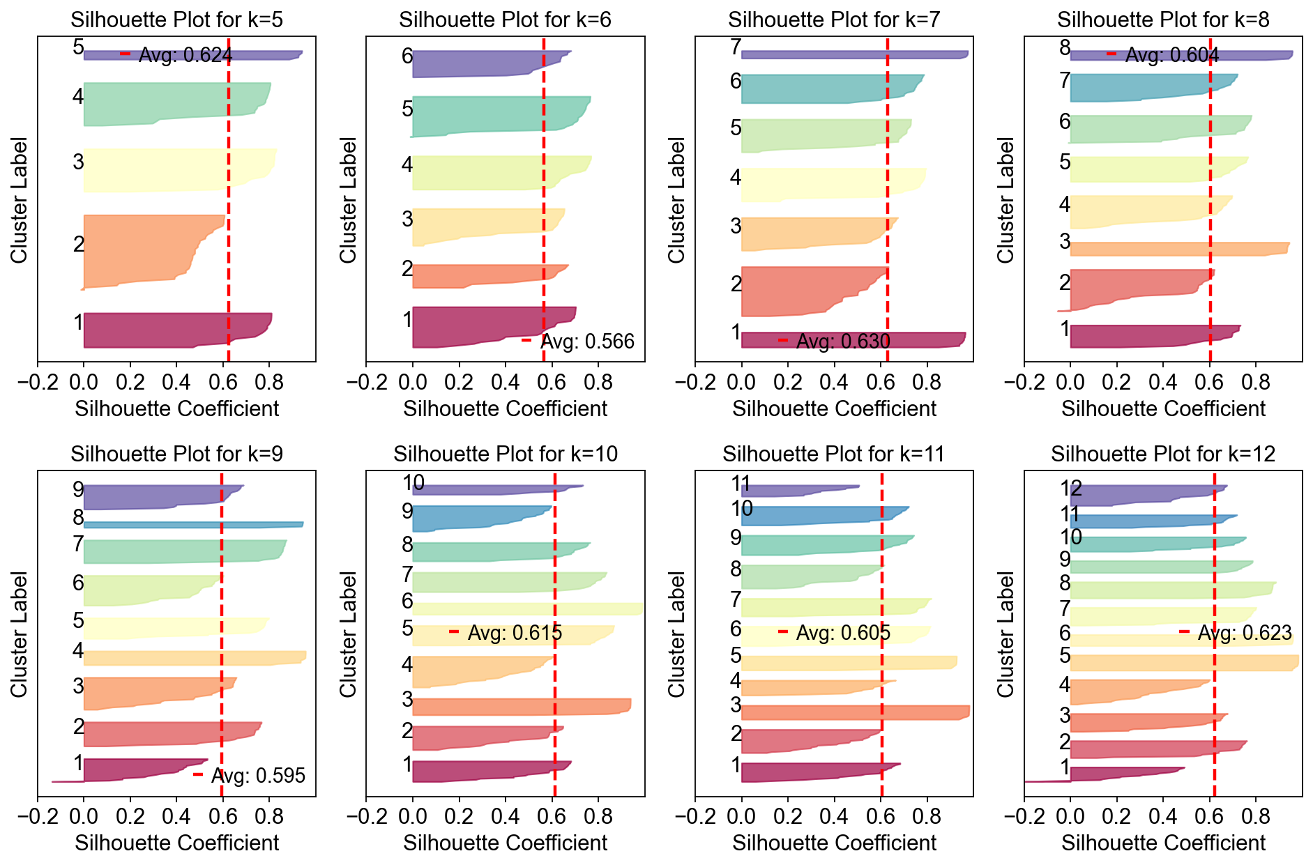
Compute the stability and error at each choice of K to see if a clear choice jumps out.

Please note that the maximum stability solution is not always the best choice depending on the application. However it is often a good starting point even if you have to investigate several choices of K

sil_data = cnmf_obj.calculate_silhouette_k(k=7, density_threshold=2.0)

print(f"Average silhouette score: {sil_data['avg_silhouette']:.4f}")
print(f"Per-sample scores: {sil_data['silhouette_values']}")
print(f"Cluster labels: {sil_data['cluster_labels']}")

Average silhouette score: 0.6299
Per-sample scores: [0.7106916  0.5630814  0.9380699  0.9647325  0.7674971  0.6231896
 0.7462224  0.37565622 0.6270655  0.06985006 0.57842237 0.7953116
 0.6916376  0.78109527 0.7101993  0.55603576 0.7441653  0.75451505
 0.5479283  0.9625558  0.39097318 0.43278462 0.97507685 0.60460097
 0.7781605  0.67471343 0.53983855 0.76693016 0.64284235 0.41358513
 0.7894957  0.5756324  0.9714798  0.54308915 0.73912    0.5916759
 0.29305577 0.5943038  0.9639678  0.75087273 0.4957365  0.7721111
 0.5499817  0.5790103  0.73023146 0.588068   0.77418405 0.18887511
 0.3828089  0.71155    0.93825644 0.66316015 0.7878561  0.9744356
 0.7274356  0.628735   0.96383363 0.63263124 0.64927    0.17515936
 0.7908563  0.59846324 0.67699015 0.37909067 0.7533861  0.27464965
 0.94846934 0.56372494 0.62612045 0.39772192 0.4309683  0.50130105
 0.5352081  0.2945753  0.7588943  0.7905221  0.7286009  0.94101614
 0.5963504  0.60703915 0.6570392  0.17053658 0.7238535  0.63654566
 0.164855   0.60783756 0.70025706 0.64824665 0.08693045 0.70052814
 0.6865447  0.5977072  0.95368004 0.7289692  0.44170102 0.7777483
 0.7743478  0.4995771  0.69891447 0.580345   0.78578705 0.3635015
 0.71654373 0.9585754  0.6125389  0.629792   0.6913672  0.4552708
 0.10541853 0.96240723 0.38784292 0.6745267  0.79051185 0.70214224
 0.84903276 0.6250461  0.509497   0.055472   0.6147614  0.49948195
 0.25953737 0.72868174 0.7900021  0.6660114  0.360943   0.6711156
 0.7861118  0.9580041  0.57364947 0.43281323 0.78196883 0.64617914
 0.50612485 0.1185286  0.7382589  0.9742657  0.67354196 0.76530886
 0.5728536  0.7114021 ]
Cluster labels: [4 2 0 6 3 1 5 1 2 4 1 3 4 5 4 2 5 3 1 0 1 1 6 2 5 4 1 3 2 1 3 4 6 1 5 1 1
 2 0 5 4 3 1 2 4 3 5 3 1 5 0 2 3 6 4 1 0 1 2 4 3 5 4 4 5 2 0 1 3 1 1 1 2 2
 5 3 4 6 1 5 2 3 4 3 3 1 5 2 4 3 4 2 0 4 1 3 5 1 5 1 3 1 4 0 2 1 3 5 2 0 2
 4 3 4 0 1 5 2 2 1 1 4 3 2 1 5 5 0 4 1 3 2 1 1 3 6 2 5 1 4]

fig, axes = plt.subplots(2,4,figsize=(12,8))
for k,ax in zip(np.arange(5,15),axes.flatten()):
    cnmf_obj.plot_silhouette_for_k(
        k=k,
        density_threshold=2.0,
        show_avg=True,
        cmap='Spectral',ax=ax
    )
plt.tight_layout()

fig=cnmf_obj.k_selection_plot(close_fig=False)

Calculating silhouette scores for K selection...

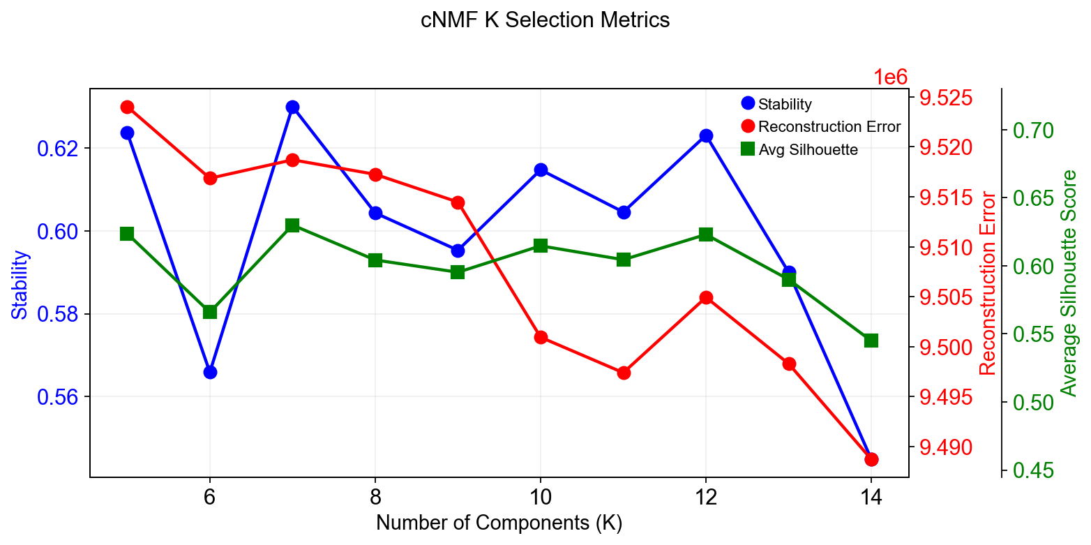
In this range, K=12 gave the most stable solution so we will begin by looking at that.

The next step computes the consensus solution for a given choice of K. We first run it without any outlier filtering to see what that looks like. Setting the density threshold to anything >= 2.00 (the maximum possible distance between two unit vectors) ensures that nothing will be filtered.

Then we run the consensus with a filter for outliers determined based on inspecting the histogram of distances between components and their nearest neighbors

selected_K = 12
density_threshold = 2.00

cnmf_obj.consensus(k=selected_K, 
                   density_threshold=density_threshold, 
                   show_clustering=True, 
                   close_clustergram_fig=False)

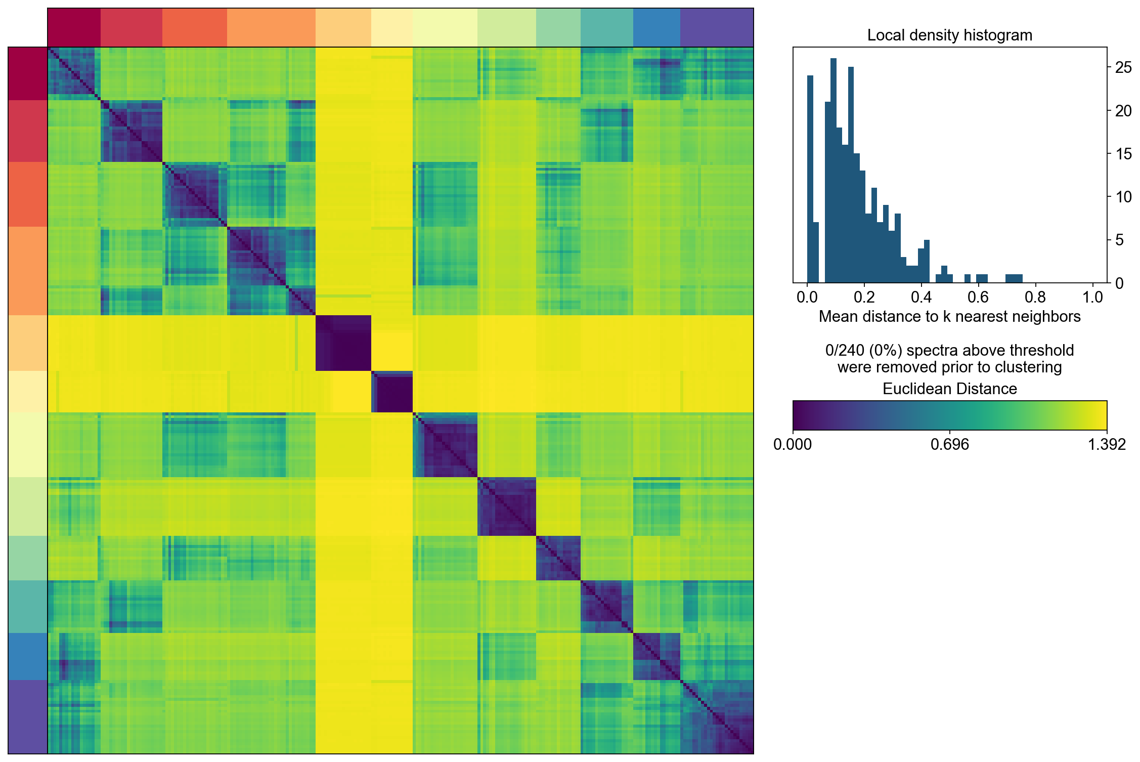
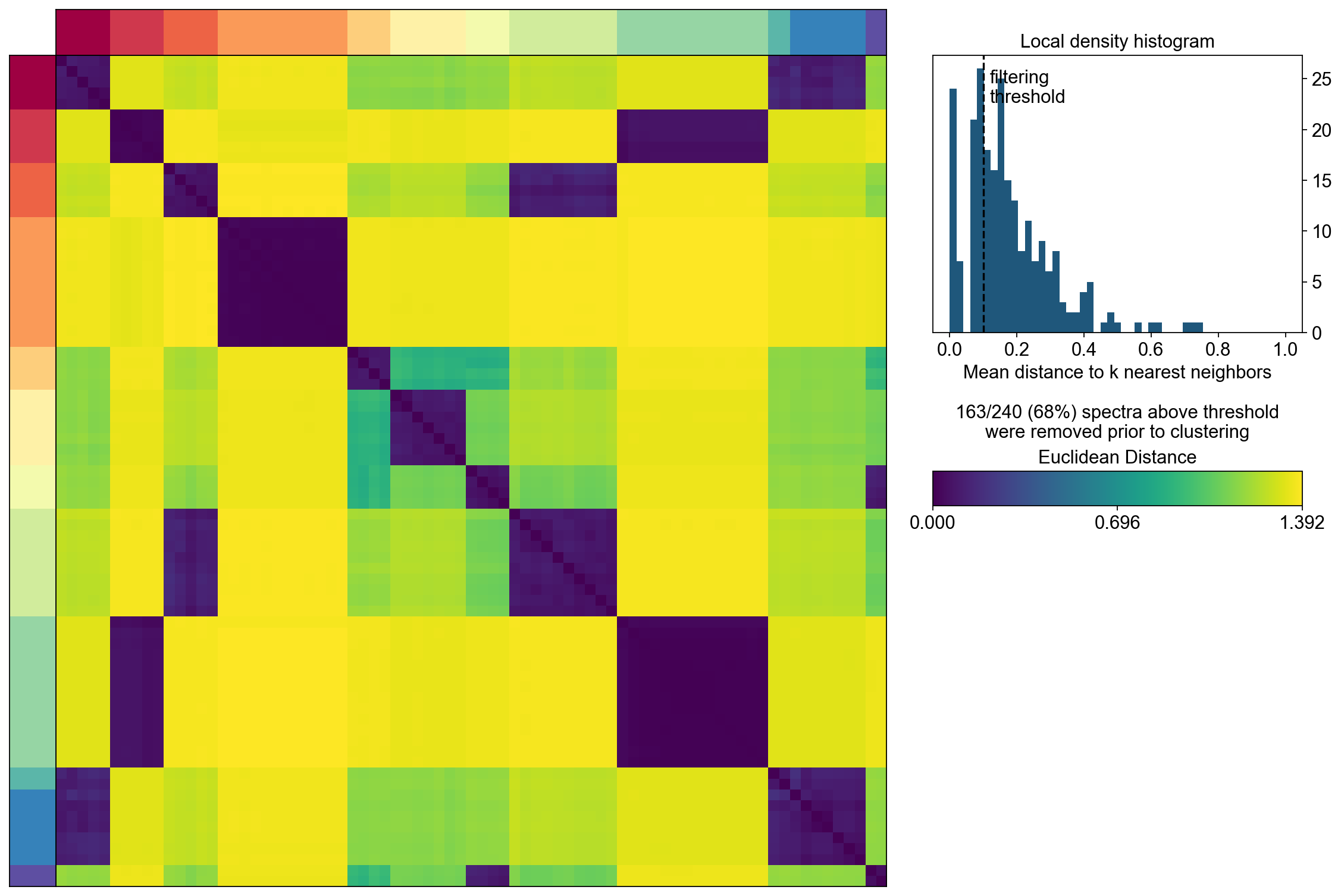
The above consensus plot shows that there is a substantial degree of concordance between the replicates with a few outliers. An outlier threshold of 0.1 seems appropriate

density_threshold = 0.10

cnmf_obj.consensus(k=selected_K, 
                   density_threshold=density_threshold, 
                   show_clustering=True, 
                   close_clustergram_fig=False)

Visualization the result

import seaborn as sns
import matplotlib.pyplot as plt
from matplotlib import patheffects

from matplotlib import gridspec
import matplotlib.pyplot as plt

width_ratios = [0.2, 4, 0.5, 10, 1]
height_ratios = [0.2, 4]
fig = plt.figure(figsize=(sum(width_ratios), sum(height_ratios)))
gs = gridspec.GridSpec(len(height_ratios), len(width_ratios), fig,
                        0.01, 0.01, 0.98, 0.98,
                       height_ratios=height_ratios,
                       width_ratios=width_ratios,
                       wspace=0, hspace=0)
            
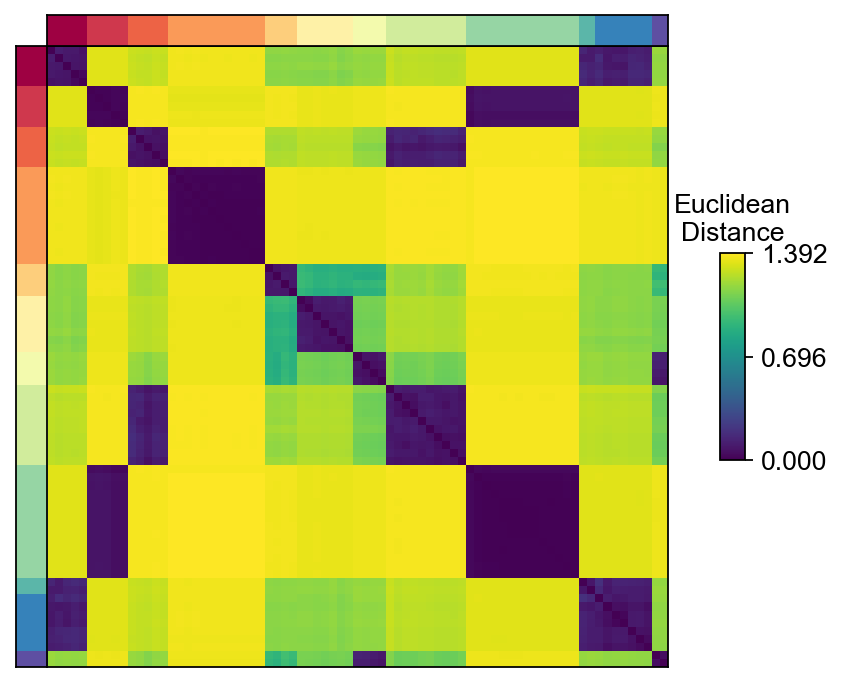
D = cnmf_obj.topic_dist[cnmf_obj.spectra_order, :][:, cnmf_obj.spectra_order]
dist_ax = fig.add_subplot(gs[1,1], xscale='linear', yscale='linear',
                                      xticks=[], yticks=[],xlabel='', ylabel='',
                                      frameon=True)
dist_im = dist_ax.imshow(D, interpolation='none', cmap='viridis',
                         aspect='auto', rasterized=True)

left_ax = fig.add_subplot(gs[1,0], xscale='linear', yscale='linear', xticks=[], yticks=[],
                xlabel='', ylabel='', frameon=True)
left_ax.imshow(cnmf_obj.kmeans_cluster_labels.values[cnmf_obj.spectra_order].reshape(-1, 1),
                            interpolation='none', cmap='Spectral', aspect='auto',
                            rasterized=True)

top_ax = fig.add_subplot(gs[0,1], xscale='linear', yscale='linear', xticks=[], yticks=[],
                xlabel='', ylabel='', frameon=True)
top_ax.imshow(cnmf_obj.kmeans_cluster_labels.values[cnmf_obj.spectra_order].reshape(1, -1),
                  interpolation='none', cmap='Spectral', aspect='auto',
                    rasterized=True)

cbar_gs = gridspec.GridSpecFromSubplotSpec(3, 3, subplot_spec=gs[1, 2],
                                   wspace=0, hspace=0)
cbar_ax = fig.add_subplot(cbar_gs[1,2], xscale='linear', yscale='linear',
    xlabel='', ylabel='', frameon=True, title='Euclidean\nDistance')
cbar_ax.set_title('Euclidean\nDistance',fontsize=12)
vmin = D.min().min()
vmax = D.max().max()
fig.colorbar(dist_im, cax=cbar_ax,
        ticks=np.linspace(vmin, vmax, 3),
        )
cbar_ax.set_yticklabels(cbar_ax.get_yticklabels(),fontsize=12)

[Text(1, 0.0, '0.000'),
 Text(1, 0.6961943507194519, '0.696'),
 Text(1, 1.3923887014389038, '1.392')]

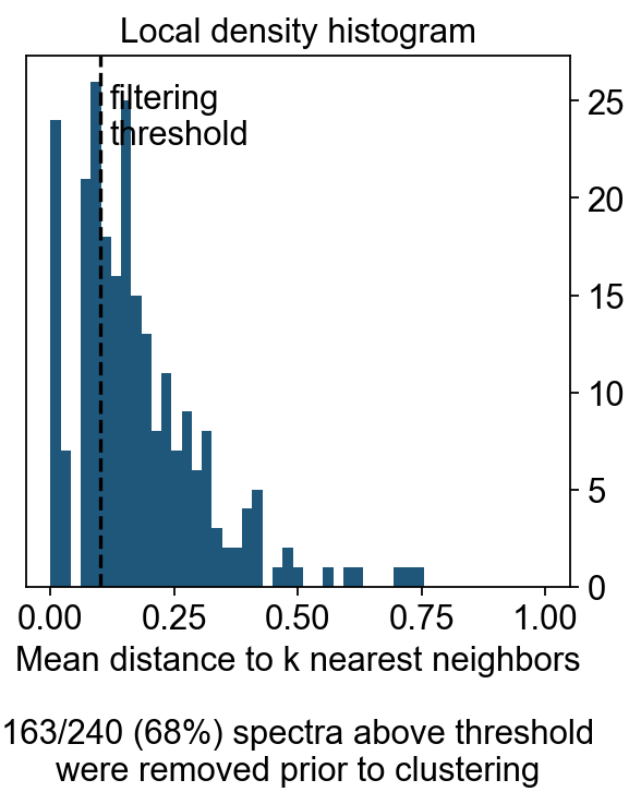
density_filter = cnmf_obj.local_density.iloc[:, 0] < density_threshold
fig, hist_ax = plt.subplots(figsize=(4,4))

#hist_ax = fig.add_subplot(hist_gs[0,0], xscale='linear', yscale='linear',
 #   xlabel='', ylabel='', frameon=True, title='Local density histogram')
hist_ax.hist(cnmf_obj.local_density.values, bins=np.linspace(0, 1, 50))
hist_ax.yaxis.tick_right()

xlim = hist_ax.get_xlim()
ylim = hist_ax.get_ylim()
if density_threshold < xlim[1]:
    hist_ax.axvline(density_threshold, linestyle='--', color='k')
    hist_ax.text(density_threshold  + 0.02, ylim[1] * 0.95, 'filtering\nthreshold\n\n', va='top')
hist_ax.set_xlim(xlim)
hist_ax.set_xlabel('Mean distance to k nearest neighbors\n\n%d/%d (%.0f%%) spectra above threshold\nwere removed prior to clustering'%(sum(~density_filter), len(density_filter), 100*(~density_filter).mean()))
hist_ax.set_title('Local density histogram')

Text(0.5, 1.0, 'Local density histogram')

Explode the cNMF result

We can load the results for a cNMF run with a given K and density filtering threshold like below

result_dict = cnmf_obj.load_results(K=selected_K, density_threshold=density_threshold)

result_dict['usage_norm'].head()

	cNMF_1	cNMF_2	cNMF_3	cNMF_4	cNMF_5	cNMF_6	cNMF_7	cNMF_8	cNMF_9	cNMF_10	cNMF_11	cNMF_12
index
AAACCTGAGAGGGATA	0.052900	0.557367	0.000422	0.021016	0.006930	0.003447	0.079662	0.082491	0.000638	0.005284	0.030603	0.159242
AAACCTGAGCCTTGAT	0.020833	0.000962	0.570114	0.043898	0.000887	0.173351	0.007137	0.132107	0.004638	0.000670	0.029395	0.016007
AAACCTGAGGCAATTA	0.000142	0.306285	0.050380	0.000632	0.017096	0.028461	0.017249	0.053764	0.000810	0.005584	0.131687	0.387909
AAACCTGCATCATCCC	0.011620	0.000740	0.142481	0.011996	0.002794	0.510735	0.001547	0.281503	0.003506	0.025785	0.005863	0.001429
AAACCTGGTAAGTGGC	0.543322	0.149150	0.003397	0.199798	0.000105	0.011512	0.023303	0.000721	0.003200	0.022096	0.025705	0.017692

result_dict['gep_scores'].head()

	1	2	3	4	5	6	7	8	9	10	11	12
index
Xkr4	-0.007757	-0.001951	0.010988	0.000303	0.000153	-0.006076	0.001394	-0.000277	0.007163	-0.000909	-0.001658	-0.001580
Mrpl15	-0.004883	0.017592	-0.018511	-0.027615	-0.021772	0.037728	0.013916	0.011741	-0.016687	0.021974	-0.005451	-0.004443
Npbwr1	0.008097	0.001318	-0.010134	-0.018095	-0.016732	0.000294	-0.003005	0.000016	0.055294	-0.001144	-0.000746	-0.001143
4732440D04Rik	0.008619	-0.005695	-0.006195	-0.013188	0.014607	0.001333	-0.008327	-0.001492	0.005998	0.000943	0.000016	-0.002278
Gm26901	-0.007764	0.026168	-0.008942	0.023266	-0.009654	-0.017616	-0.010079	0.009438	-0.008486	-0.003649	-0.001237	-0.000615

result_dict['gep_tpm'].head()

	1	2	3	4	5	6	7	8	9	10	11	12
index
Xkr4	0.000000	8.302266e-03	1.477936e-02	0.000000	1.833748e-03	3.670955e-05	8.236001e-29	1.203458e-02	0.008952	0.000000	0.000000e+00	0.002387
Mrpl15	0.010844	4.420368e-19	9.274849e-01	0.018528	5.522656e-01	7.091711e-02	1.485689e-01	3.118949e-02	0.046750	0.155717	5.128206e-14	0.662705
Npbwr1	0.016931	0.000000e+00	2.428719e-16	0.000000	9.940618e-04	4.695393e-07	0.000000e+00	0.000000e+00	0.000000	0.009431	0.000000e+00	0.000000
4732440D04Rik	0.008692	1.156003e-05	7.946806e-03	0.000000	4.226314e-02	3.767684e-02	3.580834e-02	2.182026e-12	0.000063	0.005495	3.885308e-30	0.006224
Gm26901	0.000000	3.010304e-02	3.764709e-20	0.000000	1.401298e-45	1.688556e-03	8.005813e-03	0.000000e+00	0.000000	0.000000	0.000000e+00	0.062770

result_dict['top_genes'].head()

	1	2	3	4	5	6	7	8	9	10	11	12
0	Hmgn3	Anxa2	Nnat	Grin3a	Krt7	Sox4	Gmnn	Olfm1	Ghrl	Birc5	Prph	Gpr132
1	Chgb	Cldn3	Ppp1r1a	Atoh8	1110012L19Rik	Nptx2	Mcm5	Selm	Maged2	Nusap1	Stmn2	AB124611
2	Rap1b	Krt18	Ins2	Enpp2	BC023829	Mpzl1	Pcna	Ppp1r14a	Gm11837	Cenpf	Hand2	Tyrobp
3	Cldn4	Atp1b1	Sdf2l1	Ttr	Gspt1	Bcl2	2810417H13Rik	Tmsb4x	Arg1	Plk1	Stmn4	Fcgr3
4	Pax6	Lurap1l	Iapp	Tmem171	Cck	Gadd45a	Rrm2	Shf	Irs4	Cks2	Pirt	AI662270

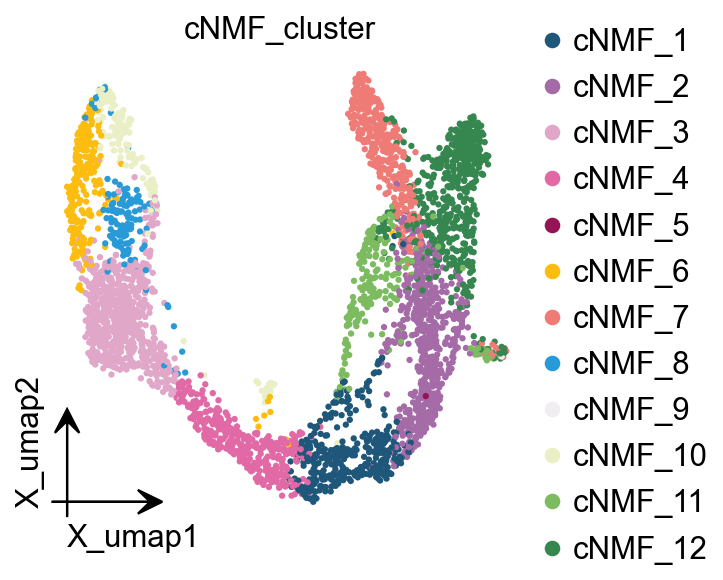
We can extract cell classes directly based on the highest cNMF in each cell, but this has the disadvantage that it will lead to mixed cell classes if the heterogeneity of our data is not as strong as it should be.

cnmf_obj.get_results(adata,result_dict)

cNMF_cluster is added to adata.obs
gene scores are added to adata.var

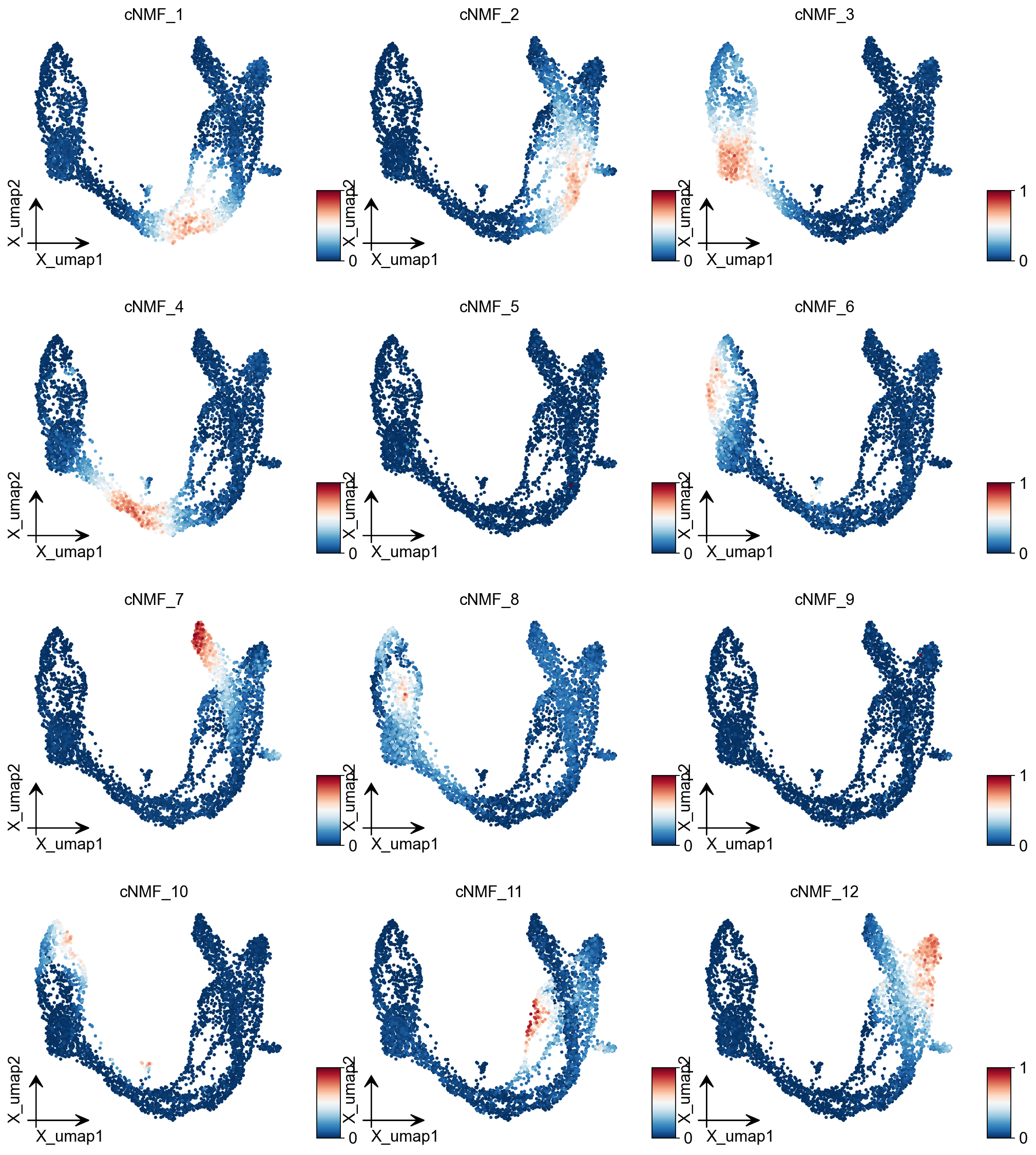
ov.pl.embedding(adata, basis='X_umap',color=result_dict['usage_norm'].columns,
           use_raw=False, ncols=3, vmin=0, vmax=1,frameon='small')

ov.pl.embedding(
    adata,
    basis="X_umap",
    color=['cNMF_cluster'],
    frameon='small',
    #title="Celltypes",
    #legend_loc='on data',
    legend_fontsize=14,
    legend_fontoutline=2,
    #size=10,
    #legend_loc=True, 
    add_outline=False, 
    #add_outline=True,
    outline_color='black',
    outline_width=1,
    show=False,
)

<Axes: title={'center': 'cNMF_cluster'}, xlabel='X_umap1', ylabel='X_umap2'>

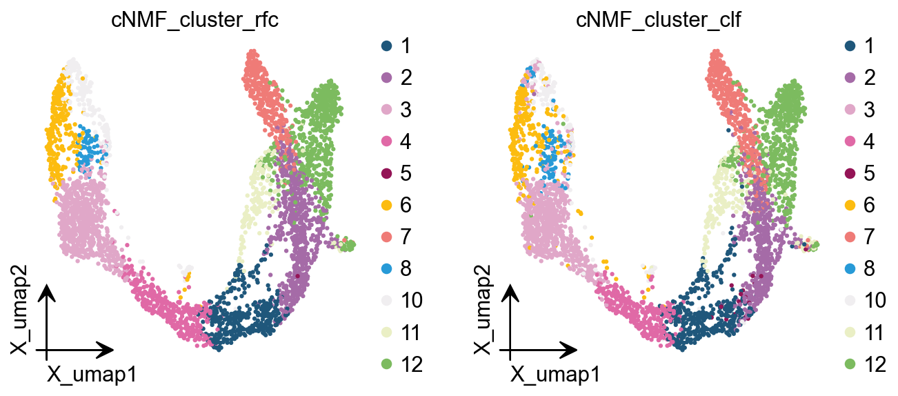
Here we are, proposing another idea of categorisation. We use cells with cNMF greater than 0.5 as a primitive class, and then train a random forest classification model, and then use the random forest classification model to classify cells with cNMF less than 0.5 to get a more accurate

cnmf_obj.get_results_rfc(adata,result_dict,
                         use_rep='scaled|original|X_pca',
                        cNMF_threshold=0.5)

Single Tree: 0.9555555555555556
Random Forest: 0.9873015873015873
cNMF_cluster_rfc is added to adata.obs
cNMF_cluster_clf is added to adata.obs

ov.pl.embedding(
    adata,
    basis="X_umap",
    color=['cNMF_cluster_rfc','cNMF_cluster_clf'],
    frameon='small',
    #title="Celltypes",
    #legend_loc='on data',
    legend_fontsize=14,
    legend_fontoutline=2,
    #size=10,
    #legend_loc=True, 
    add_outline=False, 
    #add_outline=True,
    outline_color='black',
    outline_width=1,
    show=False,
)

[<Axes: title={'center': 'cNMF_cluster_rfc'}, xlabel='X_umap1', ylabel='X_umap2'>,
 <Axes: title={'center': 'cNMF_cluster_clf'}, xlabel='X_umap1', ylabel='X_umap2'>]

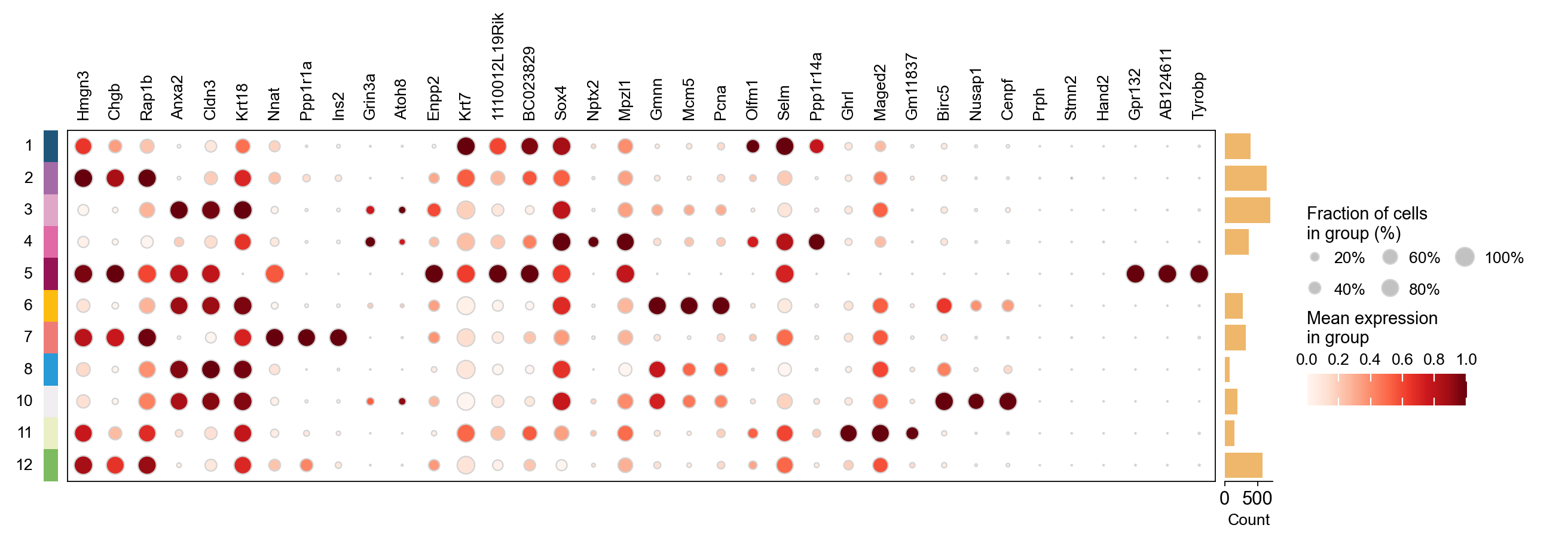
plot_genes=[]
for i in result_dict['top_genes'].columns:
    plot_genes+=result_dict['top_genes'][i][:3].values.reshape(-1).tolist()

ov.pl.dotplot(
    adata,plot_genes,
    "cNMF_cluster_rfc", dendrogram=False,standard_scale='var',
)

<marsilea.heatmap.SizedHeatmap at 0x7f84d0263e20>

Hotspot

Hotspot is a tool for identifying informative genes (and gene modules) in a single-cell dataset.

• DeTomaso D, Yosef N. Hotspot identifies informative gene modules across modalities of single-cell genomics. Cell Syst. 2021 May 19;12(5):446-456.e9. doi: 10.1016/j.cels.2021.04.005. Epub 2021 May 4. PMID: 33951459.

# to calculate the total_counts
sc.pp.calculate_qc_metrics(adata, percent_top=None, log1p=False, inplace=True)

# Create the Hotspot object and the neighborhood graph
# hotspot works a lot faster with a csc matrix!
adata.layers["counts_csc"] = adata.layers["counts"].tocsc()
hs = ov.single.Hotspot(
    adata, 
    layer_key="counts_csc", 
    model='danb', 
    latent_obsm_key="X_pca",
    umi_counts_obs_key="total_counts"
)

hs.create_knn_graph(
    weighted_graph=False, n_neighbors=30,
)

Determining informative genes

Now we compute autocorrelations for each gene, in the pca-space, to determine which genes have the most informative variation.

hs_results = hs.compute_autocorrelations(jobs=8)

hs_results.head(15)

	C	Z	Pval	FDR
Gene
Btbd17	0.735443	221.872382	0.0	0.0
Gadd45a	0.666501	213.692549	0.0	0.0
Neurog3	0.658402	208.855264	0.0	0.0
Spp1	0.806283	200.751152	0.0	0.0
Mdk	0.695210	199.681646	0.0	0.0
Rps19	0.819013	199.041836	0.0	0.0
Gnas	0.701187	192.850484	0.0	0.0
Rpl13	0.817551	192.250551	0.0	0.0
Nnat	0.780046	191.744472	0.0	0.0
Rpl18a	0.780471	191.128396	0.0	0.0
Rpl32	0.796391	190.960143	0.0	0.0
Gcg	0.603454	190.364941	0.0	0.0
Ins2	0.753340	189.588977	0.0	0.0
Ppp1r1a	0.727086	188.885836	0.0	0.0
Rps4x	0.797900	187.245979	0.0	0.0

Grouping genes into lineage-based modules

To get a better idea of what expression patterns exist, it is helpful to group the genes into modules.

Hotspot does this using the concept of “local correlations” - that is, correlations that are computed between genes between cells in the same neighborhood.

Here we avoid running the calculation for all Genes x Genes pairs and instead only run this on genes that have significant autocorrelation to begin with.

The method compute_local_correlations returns a Genes x Genes matrix of Z-scores for the significance of the correlation between genes. This object is also retained in the hs object and is used in the subsequent steps.

# Select the genes with significant lineage autocorrelation
hs_genes = hs_results.loc[hs_results.FDR < 0.05].sort_values('Z', ascending=False).head(500).index

# Compute pair-wise local correlations between these genes
lcz = hs.compute_local_correlations(hs_genes, jobs=8)

Computing pair-wise local correlation on 500 features...

Now that pair-wise local correlations are calculated, we can group genes into modules.

To do this, a convenience method is included create_modules which performs agglomerative clustering with two caveats:

• If the FDR-adjusted p-value of the correlation between two branches exceeds fdr_threshold, then the branches are not merged.

• If two branches are two be merged and they are both have at least min_gene_threshold genes, then the branches are not merged. Further genes that would join to the resulting merged module (and are therefore ambiguous) either remain unassigned (if core_only=True) or are assigned to the module with the smaller average correlations between genes, i.e. the least-dense module (if core_only=False)

The output is a Series that maps gene to module number. Unassigned genes are indicated with a module number of -1

This method was used to preserved substructure (nested modules) while still giving the analyst some control. However, since there are a lot of ways to do hierarchical clustering, you can also manually cluster using the gene-distances in hs.local_correlation_z

modules = hs.create_modules(
    min_gene_threshold=15, core_only=True, fdr_threshold=0.05
)

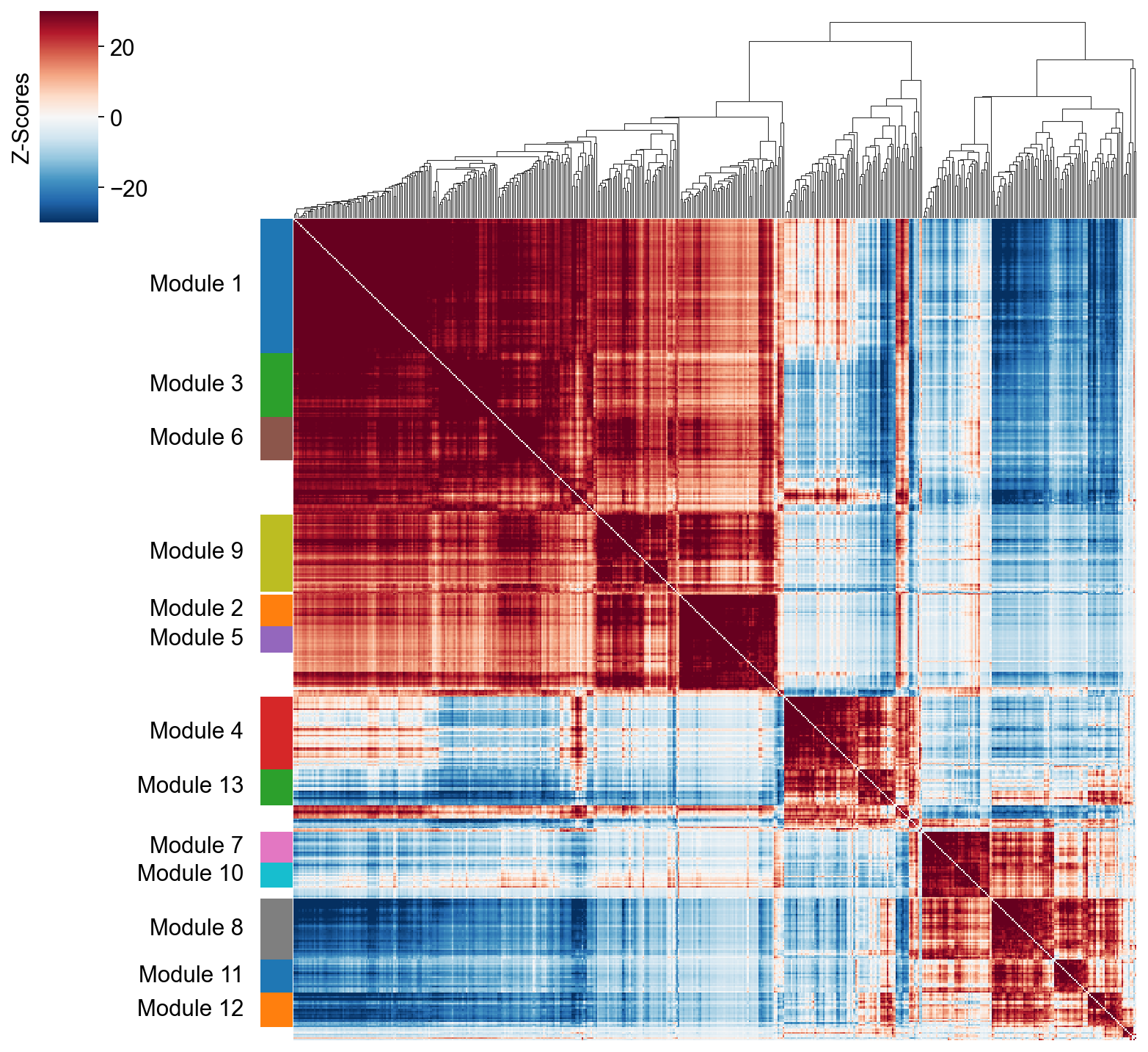
modules.value_counts()

Module
-1     93
 1     82
 9     47
 4     44
 3     39
 8     37
 6     26
 13    22
 12    21
 11    20
 7     19
 2     19
 5     16
 10    15
Name: count, dtype: int64

hs.plot_local_correlations(vmin=-30, vmax=30,)

<seaborn.matrix.ClusterGrid at 0x7f52ab7e3f10>

To explore individual genes, we can look at the genes with the top autocorrelation in a given module as these are likely the most informative.

# Show the top genes for a module

module = 4

results = hs.results.join(hs.modules)
results = results.loc[results.Module == module]

results.sort_values('Z', ascending=False).head(10)

	C	Z	Pval	FDR	Module
Gene
Btbd17	0.735443	221.872382	0.0	0.0	4.0
Gadd45a	0.666501	213.692549	0.0	0.0	4.0
Neurog3	0.658402	208.855264	0.0	0.0	4.0
Mdk	0.695210	199.681646	0.0	0.0	4.0
Tmsb4x	0.628210	187.142300	0.0	0.0	4.0
Neurod2	0.549973	183.843618	0.0	0.0	4.0
Selm	0.601179	178.700916	0.0	0.0	4.0
Smarcd2	0.577830	174.089181	0.0	0.0	4.0
Sox4	0.613079	173.945370	0.0	0.0	4.0
Btg2	0.554990	165.342505	0.0	0.0	4.0

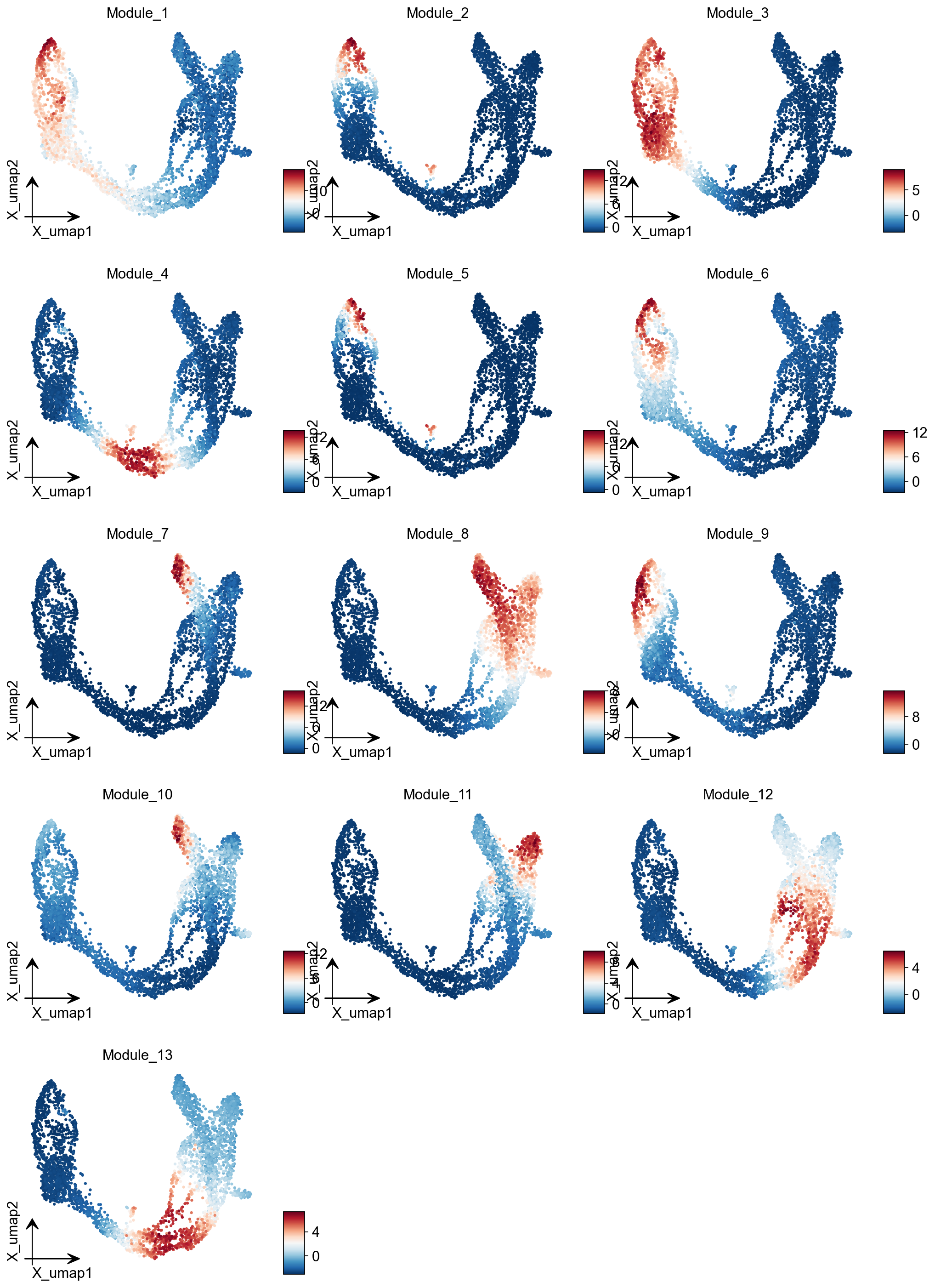
Summary Module Scores

To aid in the recognition of the general behavior of a module, Hotspot can compute aggregate module scores.

module_scores = hs.calculate_module_scores()

module_scores.head()

Computing scores for 13 modules...

	1	2	3	4	5	6	7	8	9	10	11	12	13
index
AAACCTGAGAGGGATA	-6.583796	-1.093584	-3.131375	-2.099180	-0.819142	-2.400016	-0.451105	2.504838	-2.298986	-1.439230	-0.739708	3.368700	0.531080
AAACCTGAGCCTTGAT	7.663903	-0.765588	6.610663	-2.388122	-0.689135	2.296545	-1.217827	-3.391921	0.921212	-0.813991	-1.694216	-2.358554	-2.625691
AAACCTGAGGCAATTA	-6.066218	-1.212847	-3.005648	-2.684893	-0.703958	-2.226183	-0.702572	2.636014	-2.243965	-0.119376	0.899747	2.736469	-0.274772
AAACCTGCATCATCCC	11.594423	4.786089	5.015609	-2.241397	0.848967	8.482152	-0.886003	-3.327994	12.943623	0.456323	-1.689177	-2.565122	-2.858705
AAACCTGGTAAGTGGC	-3.090054	-1.036188	-3.197947	5.563916	-0.793746	-2.413544	-1.378844	-2.149192	-2.072845	-2.134279	-1.460957	-0.137338	6.417286

module_cols = []
for c in module_scores.columns:
    key = f"Module_{c}"
    adata.obs[key] = module_scores[c]
    module_cols.append(key)

ov.pl.embedding(adata, basis='X_umap',color=module_cols,
           use_raw=False, ncols=3, frameon='small')