Identify the driver regulators of cell fate decisions

CEFCON is a computational tool for deciphering driver regulators of cell fate decisions from single-cell RNA-seq data. It takes a prior gene interaction network and expression profiles from scRNA-seq data associated with a given developmental trajectory as inputs, and consists of three main components, including cell-lineage-specific gene regulatory network (GRN) construction, driver regulator identification and regulon-like gene module (RGM) identification.

Check out (Wang et al., Nature Communications, 2023) for the detailed methods and applications.

Code: https://github.com/WPZgithub/CEFCON

import omicverse as ov
#print(f"omicverse version: {ov.__version__}")
import scanpy as sc
#print(f"scanpy version: {sc.__version__}")
import pandas as pd
from tqdm.auto import tqdm
ov.plot_set()

   ____            _     _    __                  
  / __ \____ ___  (_)___| |  / /__  _____________ 
 / / / / __ `__ \/ / ___/ | / / _ \/ ___/ ___/ _ \ 
/ /_/ / / / / / / / /__ | |/ /  __/ /  (__  )  __/ 
\____/_/ /_/ /_/_/\___/ |___/\___/_/  /____/\___/                                              

Version: 1.5.6, Tutorials: https://omicverse.readthedocs.io/

Data loading and processing

Here, we use the mouse hematopoiesis data provided by Nestorowa et al. (2016, Blood).

The scRNA-seq data requires processing to extract lineage information for the CEFCON analysis. Please refer to the original notebook for detailed instructions on preprocessing scRNA-seq data.

adata = ov.single.mouse_hsc_nestorowa16()
adata

Load mouse_hsc_nestorowa16_v0.h5ad

AnnData object with n_obs × n_vars = 1645 × 3000
    obs: 'E_pseudotime', 'GM_pseudotime', 'L_pseudotime', 'label_info', 'n_genes', 'leiden', 'cell_type_roughly', 'cell_type_finely'
    var: 'n_cells', 'highly_variable', 'means', 'dispersions', 'dispersions_norm', 'E_pseudotime_logFC', 'GM_pseudotime_logFC', 'L_pseudotime_logFC'
    uns: 'cell_type_finely_colors', 'cell_type_roughly_colors', 'draw_graph', 'hvg', 'leiden', 'leiden_colors', 'lineages', 'neighbors', 'pca', 'tsne', 'umap'
    obsm: 'X_draw_graph_fa', 'X_pca'
    varm: 'PCs'
    layers: 'raw_count'
    obsp: 'connectivities', 'distances'

CEFCON fully exploit an available global and context-free gene interaction network as prior knowledge, from which we extract the cell-lineage-specific gene interactions according to the gene expression profiles derived from scRNA-seq data associated with a given developmental trajectory.

You can download the prior network in the zenodo. CEFCON only provides the prior network for human and mosue data anaylsis. For other species, you should provide the prior network mannully.

The author of CEFCON has provided several prior networks here; however, ‘nichenet’ yields the best results.

prior_network = ov.single.load_human_prior_interaction_network(dataset='nichenet') 

Load the prior gene interaction network: nichenet. #Genes: 25345, #Edges: 5290993

In the scRNA-seq analysis of human data, you should not run this step. Running it may change the gene symbol and result in errors.

# Convert the gene symbols of the prior gene interaction network to the mouse gene symbols
prior_network = ov.single.convert_human_to_mouse_network(prior_network,server_name='asia') 
prior_network

Convert genes of the prior interaction network to mouse gene symbols:
Server 'http://asia.ensembl.org/biomart/' is OK
The converted prior gene interaction network: #Genes: 18579, #Edges: 5029532

	from	to
0	Klf2	Dlgap1
2	Klf2	Bhlhe40
3	Klf2	Rps6ka1
4	Klf2	Pxn
5	Klf2	Ube2v1
...	...	...
837982	Zranb1	Zfp141
837983	Zranb1	Zfy1
837984	Zranb1	Zfy2
837987	Zscan21	Zfy1
837988	Zscan21	Zfy2

5029532 rows × 2 columns

prior_network.to_csv('result/combined_network_Mouse.txt.gz',sep='\t')

Alternatively, you can directly specify the file path of the input prior interaction network and import the specified file.

#prior_network = './Reference_Networks/combined_network_Mouse.txt'
prior_network=ov.read('result/combined_network_Mouse.txt.gz',index_col=0)

Training CEFCON model

We recommend using GRUOBI to solve the integer linear programming (ILP) problem when identifying driver genes. GUROBI is a commercial solver that requires licenses to run. Thankfully, it provides free licenses in academia, as well as trial licenses outside academia. If there is no problem about the licenses, you need to install the gurobipy package.

If difficulties arise while using GUROBI, the non-commercial solver, SCIP, will be employed as an alternative. But the use of SCIP does not come with a guarantee of achieving a successful solutio

By default, the program will verify the availability of GRUOBI. If GRUOBI is not accessible, it will automatically switch the solver to SCIP.

CEFCON_obj = ov.single.pyCEFCON(adata, prior_network, repeats=5, solver='GUROBI')
CEFCON_obj

<omicverse.single._cefcon.pyCEFCON at 0x7f7214e73c40>

Construct cell-lineage-specific GRNs

CEFCON_obj.preprocess()

Start data preparation

[0] - Data loading and preprocessing...
Consider the input data with 3 lineages:
  Lineage - E_pseudotime:
    2935 extra edges (Spearman correlation > 0.6) are added into the prior gene interaction network.
    Total number of edges: 90036.
    n_genes × n_cells = 2803 × 1065
  Lineage - GM_pseudotime:
    100 extra edges (Spearman correlation > 0.6) are added into the prior gene interaction network.
    Total number of edges: 90136.
    n_genes × n_cells = 2803 × 882
  Lineage - L_pseudotime:
    4 extra edges (Spearman correlation > 0.6) are added into the prior gene interaction network.
    Total number of edges: 90140.
    n_genes × n_cells = 2803 × 843

Lineage-by-lineage computation:

CEFCON_obj.train()

Start model training

[1] - Constructing cell-lineage-specific GRN...
  Lineage - E_pseudotime:
[1] - Constructing cell-lineage-specific GRN...
  Lineage - GM_pseudotime:
[1] - Constructing cell-lineage-specific GRN...
  Lineage - L_pseudotime:
Finish model training

# Idenytify driver regulators for each lineage
CEFCON_obj.predicted_driver_regulators()

Start predict lineage - E_pseudotime:
Start calculate gene influence score - E_pseudotime:
Start calculate gene driver regulators - E_pseudotime:
[2] - Identifying driver regulators...
  Solving MFVS problem...
    176 critical nodes are found.
    0 nodes left after graph reduction operation.
  176 MFVS driver genes are found.
  Solving MDS problem...
    15 critical nodes are found.
    1124 nodes left after graph reduction operation.
    Solving the Integer Linear Programming problem on the reduced graph...
      Solving by GUROBI...(optimal value with GUROBI:116.0,  status:optimal)
  131 MDS driver genes are found.
Start predict lineage - GM_pseudotime:
Start calculate gene influence score - GM_pseudotime:
Start calculate gene driver regulators - GM_pseudotime:
[2] - Identifying driver regulators...
  Solving MFVS problem...
    232 critical nodes are found.
    0 nodes left after graph reduction operation.
  232 MFVS driver genes are found.
  Solving MDS problem...
    18 critical nodes are found.
    1572 nodes left after graph reduction operation.
    Solving the Integer Linear Programming problem on the reduced graph...
      Solving by GUROBI...(optimal value with GUROBI:206.0,  status:optimal)
  224 MDS driver genes are found.
Start predict lineage - L_pseudotime:
Start calculate gene influence score - L_pseudotime:
Start calculate gene driver regulators - L_pseudotime:
[2] - Identifying driver regulators...
  Solving MFVS problem...
    180 critical nodes are found.
    4 nodes left after graph reduction operation.
    Solving the Integer Linear Programming problem on the reduced graph...
      Solving by GUROBI...(optimal value with GUROBI:2.0,  status:optimal)
  182 MFVS driver nodes are found.
  Solving MDS problem...
    18 critical nodes are found.
    1747 nodes left after graph reduction operation.
    Solving the Integer Linear Programming problem on the reduced graph...
      Solving by GUROBI...(optimal value with GUROBI:300.0,  status:optimal)
  318 MDS driver genes are found.

We can find out the driver regulators identified by CEFCON.

CEFCON_obj.cefcon_results_dict['E_pseudotime'].driver_regulator.head()

	influence_score	is_driver_regulator	is_MFVS_driver	is_MDS_driver	is_TF
JUN	7.352254	True	True	True	True
GATA1	7.071392	True	True	True	True
FOS	6.930125	True	True	True	True
GATA2	6.683559	True	False	True	True
MEIS1	5.851068	True	True	True	True

CEFCON_obj.predicted_RGM()

Start calculate regulon-like gene modules - E_pseudotime:
[3] - Identifying regulon-like gene modules...
Done!
Start calculate regulon-like gene modules - GM_pseudotime:
[3] - Identifying regulon-like gene modules...
Done!
Start calculate regulon-like gene modules - L_pseudotime:
[3] - Identifying regulon-like gene modules...
Done!
Finish predicted

Downstream analysis

CEFCON_obj.cefcon_results_dict['E_pseudotime']

CefconResults object with n_cells * n_genes = 1065 * 2748, n_edges = 22424
    name: E_pseudotime
    expression_data: yes
    network: DiGraph with 2748 nodes and 22399 edges
    gene_embedding: # dimension = 64
    influence_score: yes
    driver_regulator: yes
    gene_cluster: None
    RGMs_AUCell_dict: yes

lineage = 'E_pseudotime'
result = CEFCON_obj.cefcon_results_dict[lineage]

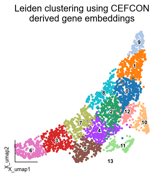
Plot gene embedding clusters

gene_ad=sc.AnnData(result.gene_embedding)
sc.pp.neighbors(gene_ad, n_neighbors=30, use_rep='X')
# Higher resolutions lead to more communities, while lower resolutions lead to fewer communities.
sc.tl.leiden(gene_ad, resolution=1)
sc.tl.umap(gene_ad, n_components=2, min_dist=0.3)

computing neighbors
    finished: added to `.uns['neighbors']`
    `.obsp['distances']`, distances for each pair of neighbors
    `.obsp['connectivities']`, weighted adjacency matrix (0:00:01)
running Leiden clustering
    finished: found 14 clusters and added
    'leiden', the cluster labels (adata.obs, categorical) (0:00:01)
computing UMAP
    finished: added
    'X_umap', UMAP coordinates (adata.obsm) (0:00:06)

ov.utils.embedding(gene_ad,basis='X_umap',legend_loc='on data',
                       legend_fontsize=8, legend_fontoutline=2,
                  color='leiden',frameon='small',title='Leiden clustering using CEFCON\nderived gene embeddings')

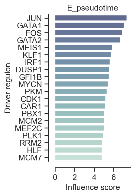
Plot influence scores of driver regulators

import matplotlib.pyplot as plt
import seaborn as sns
data_for_plot = result.driver_regulator[result.driver_regulator['is_driver_regulator']]
data_for_plot = data_for_plot[0:20]

plt.figure(figsize=(2, 20 * 0.2))
sns.set_theme(style='ticks', font_scale=0.5)

ax = sns.barplot(x='influence_score', y=data_for_plot.index, data=data_for_plot, orient='h',
                 palette=sns.color_palette(f"ch:start=.5,rot=-.5,reverse=1,dark=0.4", n_colors=20))
ax.set_title(result.name)
ax.set_xlabel('Influence score')
ax.set_ylabel('Driver regulators')

ax.spines['left'].set_position(('outward', 10))
ax.spines['bottom'].set_position(('outward', 10))
plt.xticks(fontsize=12)
plt.yticks(fontsize=12)

plt.grid(False)
#设置spines可视化情况
ax.spines['top'].set_visible(False)
ax.spines['right'].set_visible(False)
ax.spines['bottom'].set_visible(True)
ax.spines['left'].set_visible(True)

plt.title('E_pseudotime',fontsize=12)
plt.xlabel('Influence score',fontsize=12)
plt.ylabel('Driver regulon',fontsize=12)

sns.despine()

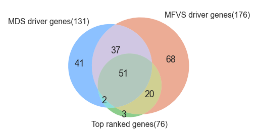
result.plot_driver_genes_Venn()

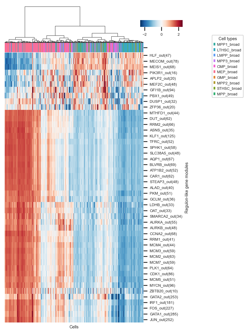
Plot heat map of the activity matrix of RGMs

adata_lineage = adata[adata.obs_names[adata.obs[result.name].notna()],:]

result.plot_RGM_activity_heatmap(cell_label=adata_lineage.obs['cell_type_finely'],
                                 type='out',col_cluster=True,bbox_to_anchor=(1.48, 0.25))

<Figure size 320x320 with 0 Axes>