Celltype annotation migration(mapping) with TOSICA
We know that when all samples cannot be obtained at the same time, it would be desirable to classify the cell types on the first batch of data and use them to annotate the data obtained later or to be obtained in the future with the same standard, without the need to processing and mapping them together again.
So migration(mapping) the reference cell annotation is necessary. This tutorial focuses on how to migration(mapping) the cell annotation from reference scRNA-seq atlas to new scRNA-seq data.
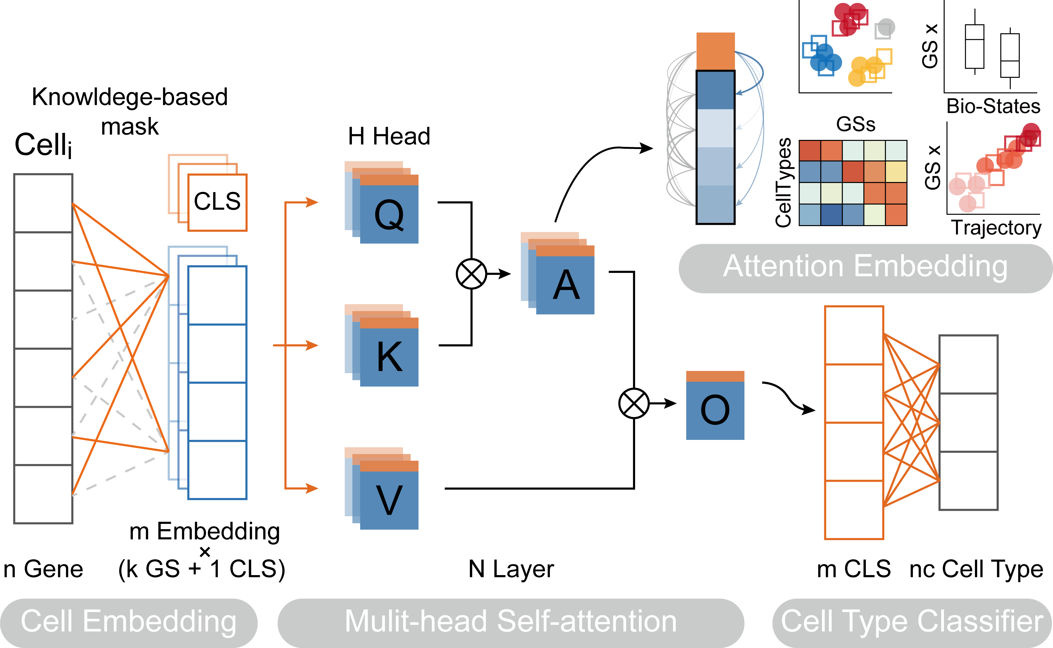
Paper: Transformer for one stop interpretable cell type annotation
Code: https://github.com/JackieHanLab/TOSICA
Colab_Reproducibility:https://colab.research.google.com/drive/1BjPEG-kLAgicP8iQvtVtpzzbIOmk1X23?usp=sharing
import omicverse as ov
import scanpy as sc
ov.utils.ov_plot_set()
Loading data
demo_train.h5ad: Braon(GSE84133) and Muraro(GSE85241)demo_test.h5ad: xin(GSE81608), segerstolpe(E-MTAB-5061) and Lawlor(GSE86473)
They can be downloaded at https://figshare.com/projects/TOSICA_demo/158489.
ref_adata = sc.read('demo_train.h5ad')
ref_adata = ref_adata[:,ref_adata.var_names]
print(ref_adata)
print(ref_adata.obs.Celltype.value_counts())
View of AnnData object with n_obs × n_vars = 10600 × 3000
    obs: 'Celltype'
    var: 'Gene Symbol'
alpha          3136
beta           2966
ductal         1290
acinar         1144
delta           793
PSC             524
PP              356
endothelial     273
macrophage       52
mast             25
epsilon          21
schwann          13
t_cell            7
Name: Celltype, dtype: int64
query_adata = sc.read('demo_test.h5ad')
query_adata = query_adata[:,ref_adata.var_names]
print(query_adata)
print(query_adata.obs.Celltype.value_counts())
View of AnnData object with n_obs × n_vars = 4218 × 3000
    obs: 'Celltype'
    var: 'Gene Symbol'
alpha           2011
beta            1006
ductal           414
PP               282
acinar           209
delta            188
PSC               73
endothelial       16
epsilon            7
mast               7
MHC class II       5
Name: Celltype, dtype: int64
We need to select the same gene training and predicting the celltype
ref_adata.var_names_make_unique()
query_adata.var_names_make_unique()
ret_gene=list(set(query_adata.var_names) & set(ref_adata.var_names))
len(ret_gene)
query_adata=query_adata[:,ret_gene]
ref_adata=ref_adata[:,ret_gene]
print(f"The max of ref_adata is {ref_adata.X.max()}, query_data is {query_adata.X.max()}",)
The max of ref_adata is 8.72524356842041, query_data is 9.2676362991333
By comparing the maximum values of the two data, we can see that the data has been normalised sc.pp.normalize_total and logarithmised sc.pp.log1p. The same treatment is applied to the data when we use our own data for analysis.
Download Genesets
Here, we need to download the genesets as pathway at first. You can use ov.utils.download_tosica_gmt() to download automatically or manual download from:
‘reactome’:’https://figshare.com/ndownloader/files/41460051’,
‘m_GO_bp’:’https://figshare.com/ndownloader/files/41460060’,
‘m_reactome’:’https://figshare.com/ndownloader/files/41460054’,
‘immune’:’https://figshare.com/ndownloader/files/41460063’,
ov.utils.download_tosica_gmt()
Initialisation the TOSICA model
We first need to train the TOSICA model on the REFERENCE dataset, where omicverse provides a simple class pyTOSICA, and all subsequent operations can be done with pyTOSICA. We need to set the parameters for model initialisation.
adata: the reference adata objectgmt_path: default pre-prepared mask or path to .gmt files. you can useov.utils.download_tosica_gmt()to obtain the genesetsdepth: the depth of transformer model, When it is set to 2, a memory leak may occurlabel_name: the reference key of celltype inadata.obsproject_path: the save path of TOSICA modelbatch_size: indicates the number of cells passed to the programme for training in a single pass
tosica_obj=ov.single.pyTOSICA(adata=ref_adata,
                              gmt_path='genesets/GO_bp.gmt', depth=1,
                              label_name='Celltype',
                              project_path='hGOBP_demo',
                              batch_size=8)
cuda:0
Mask loaded!
Training the TOSICA model
There’re 4 arguments to set when training the TOSICA model.
pre_weights: The path of the pre-trained weights.
lr: The learning rate.
epochs: The number of epochs.
lrf: The learning rate of the last layer.
tosica_obj.train(epochs=5)
Model builded!
Training finished!
Transformer(
  (feature_embed): FeatureEmbed(
    (fe): CustomizedLinear(input_features=3000, output_features=14400, bias=True)
    (norm): Identity()
  )
  (blocks): ModuleList(
    (0): Block(
      (norm1): LayerNorm((48,), eps=1e-06, elementwise_affine=True)
      (attn): Attention(
        (qkv): Linear(in_features=48, out_features=144, bias=True)
        (attn_drop): Dropout(p=0.5, inplace=False)
        (proj): Linear(in_features=48, out_features=48, bias=True)
        (proj_drop): Dropout(p=0.5, inplace=False)
      )
      (drop_path): Identity()
      (norm2): LayerNorm((48,), eps=1e-06, elementwise_affine=True)
      (mlp): Mlp(
        (fc1): Linear(in_features=48, out_features=192, bias=True)
        (act): GELU(approximate='none')
        (fc2): Linear(in_features=192, out_features=48, bias=True)
        (drop): Dropout(p=0.5, inplace=False)
      )
    )
  )
  (norm): LayerNorm((48,), eps=1e-06, elementwise_affine=True)
  (pre_logits): Identity()
  (head): Linear(in_features=48, out_features=13, bias=True)
)
We can use .save to store the TOSICA model in project_path
tosica_obj.save()
Model saved!
The model can be loaded from project_path automatically.
tosica_obj.load()
Model loaded!
Update with query
new_adata=tosica_obj.predicted(pre_adata=query_adata)
0
4218
Visualize the reference and mapping
We first compute the lower dimensional space of query_data, where we use omicverse’s preprocessing method as well as the mde method for dimensionality reduction
To visualize the PCA’s embeddings, we use the pymde package wrapper in omicverse. This is an alternative to UMAP that is GPU-accelerated.
ov.pp.scale(query_adata)
ov.pp.pca(query_adata,layer='scaled',n_pcs=50)
sc.pp.neighbors(query_adata, n_neighbors=15, n_pcs=50,
               use_rep='scaled|original|X_pca')
query_adata.obsm["X_mde"] = ov.utils.mde(query_adata.obsm["scaled|original|X_pca"])
query_adata
computing neighbors
    finished: added to `.uns['neighbors']`
    `.obsp['distances']`, distances for each pair of neighbors
    `.obsp['connectivities']`, weighted adjacency matrix (0:00:02)
AnnData object with n_obs × n_vars = 4218 × 3000
    obs: 'Celltype'
    var: 'Gene Symbol'
    uns: 'scaled|original|pca_var_ratios', 'scaled|original|cum_sum_eigenvalues', 'neighbors'
    obsm: 'scaled|original|X_pca', 'X_mde'
    varm: 'scaled|original|pca_loadings'
    layers: 'scaled', 'lognorm'
    obsp: 'distances', 'connectivities'
Since new_adata and query_adata have the same cells, their low-dimensional spaces are also the same. So we proceed directly to the assignment operation.
new_adata.obsm=query_adata[new_adata.obs.index].obsm.copy()
new_adata.obsp=query_adata[new_adata.obs.index].obsp.copy()
new_adata
AnnData object with n_obs × n_vars = 4218 × 299
    obs: 'Prediction', 'Probability', 'Celltype'
    obsm: 'scaled|original|X_pca', 'X_mde'
    obsp: 'distances', 'connectivities'
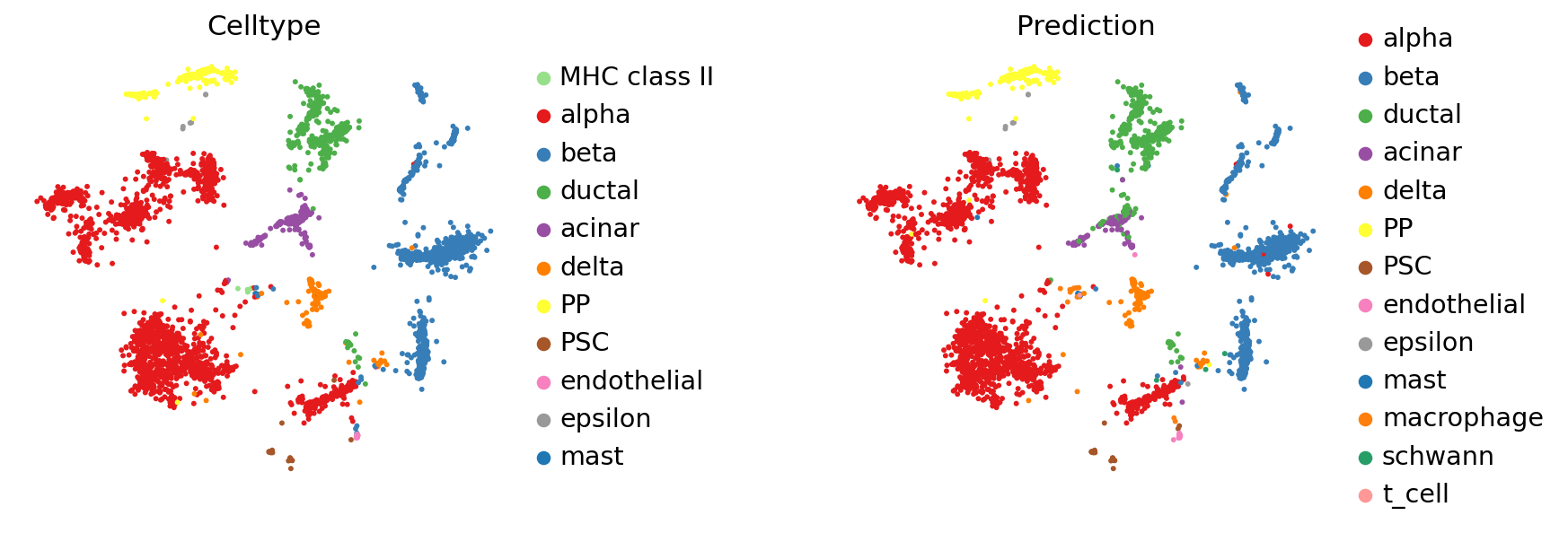
Since the predicted cell types are not exactly the same as the original cell types, the colours are not exactly the same. For the visualisation effect, we manually set the colour of the predicted cell type with the original cell type.
import numpy as np
col = np.array([
"#98DF8A","#E41A1C" ,"#377EB8", "#4DAF4A" ,"#984EA3" ,"#FF7F00" ,"#FFFF33" ,"#A65628" ,"#F781BF" ,"#999999","#1F77B4","#FF7F0E","#279E68","#FF9896"
]).astype('<U7')

celltype = ("alpha","beta","ductal","acinar","delta","PP","PSC","endothelial","epsilon","mast","macrophage","schwann",'t_cell')
new_adata.obs['Prediction'] = new_adata.obs['Prediction'].astype('category')
new_adata.obs['Prediction'] = new_adata.obs['Prediction'].cat.reorder_categories(list(celltype))
new_adata.uns['Prediction_colors'] = col[1:]

celltype = ("MHC class II","alpha","beta","ductal","acinar","delta","PP","PSC","endothelial","epsilon","mast")
new_adata.obs['Celltype'] = new_adata.obs['Celltype'].astype('category')
new_adata.obs['Celltype'] = new_adata.obs['Celltype'].cat.reorder_categories(list(celltype))
new_adata.uns['Celltype_colors'] = col[:11]
sc.pl.embedding(
    new_adata,
    basis="X_mde",
    color=['Celltype', 'Prediction'],
    frameon=False,
    #ncols=1,
    wspace=0.5,
    #palette=ov.utils.pyomic_palette()[11:],
    show=False,
)
[<AxesSubplot: title={'center': 'Celltype'}, xlabel='X_mde1', ylabel='X_mde2'>,
 <AxesSubplot: title={'center': 'Prediction'}, xlabel='X_mde1', ylabel='X_mde2'>]
Pathway attention
TOSICA has another special feature, which is the ability to computationally use self-attention mechanisms to find pathways associated with cell types. Here we demonstrate the approach of this downstream analysis.
We first need to filter out the predicted types of cells with cell counts less than 5.
cell_idx=new_adata.obs['Prediction'].value_counts()[new_adata.obs['Prediction'].value_counts()<5].index
new_adata=new_adata[~new_adata.obs['Prediction'].isin(cell_idx)]
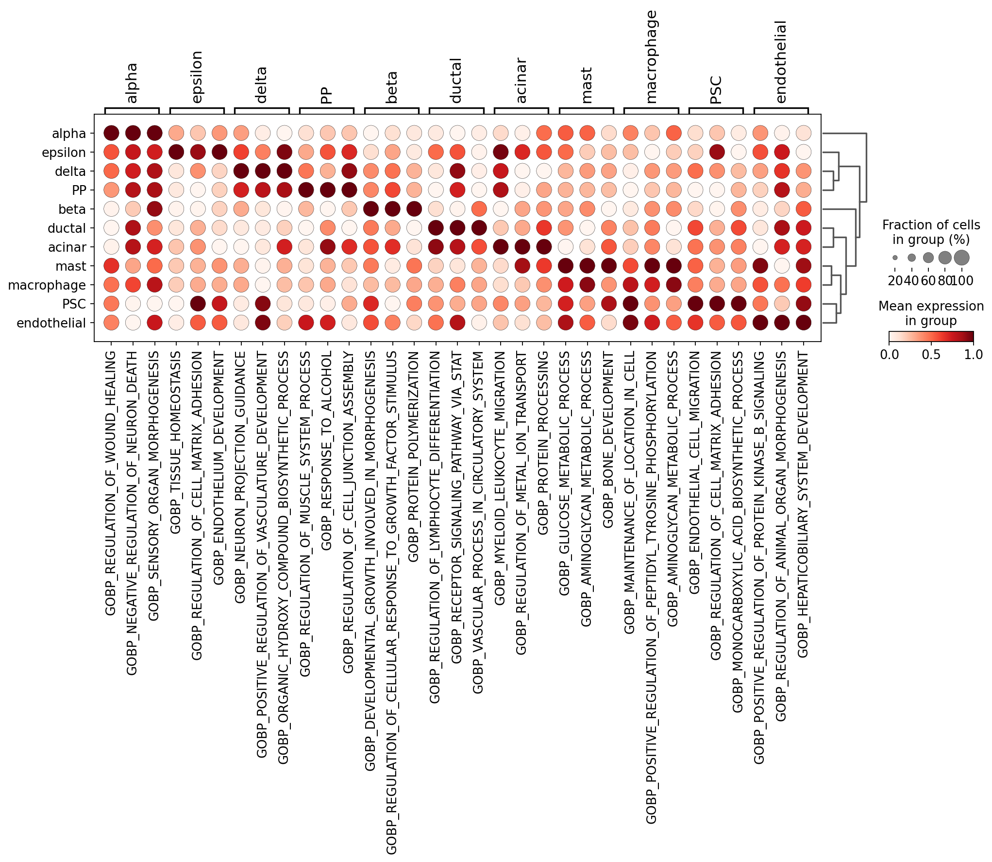
We then used sc.tl.rank_genes_groups to calculate the differential pathways with the highest attention across cell types. This differential pathway is derived from the gmt genesets used for the previous calculation.
sc.tl.rank_genes_groups(new_adata, 'Prediction', method='wilcoxon')
ranking genes
    finished: added to `.uns['rank_genes_groups']`
    'names', sorted np.recarray to be indexed by group ids
    'scores', sorted np.recarray to be indexed by group ids
    'logfoldchanges', sorted np.recarray to be indexed by group ids
    'pvals', sorted np.recarray to be indexed by group ids
    'pvals_adj', sorted np.recarray to be indexed by group ids (0:00:00)
sc.pl.rank_genes_groups_dotplot(new_adata,
                                n_genes=3,standard_scale='var',)
If you want to get the cell-specific pathway, you can use sc.get.rank_genes_groups_df to get.
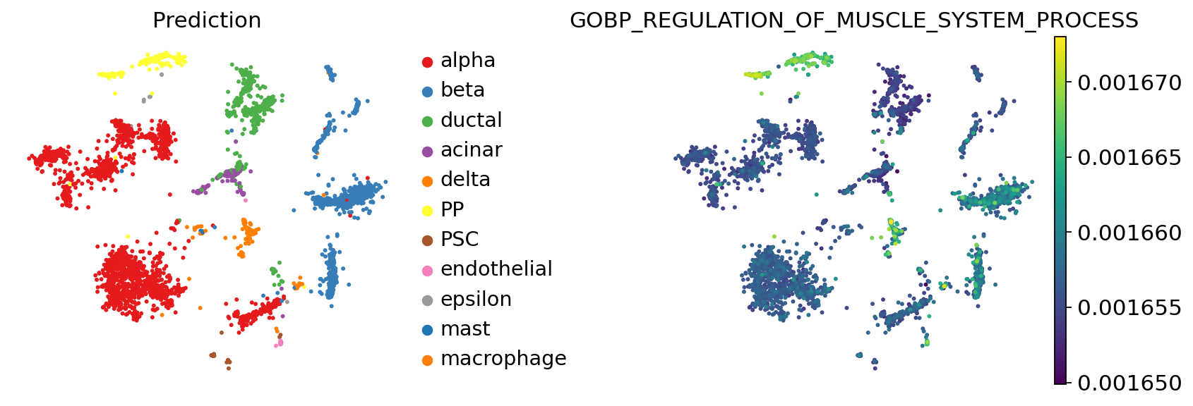
For example, we would like to obtain the pathway with the highest attention for the cell type PP
degs = sc.get.rank_genes_groups_df(new_adata, group='PP', key='rank_genes_groups',
                                            pval_cutoff=0.05)
degs.head()
| names | scores | logfoldchanges | pvals | pvals_adj | |
|---|---|---|---|---|---|
| 0 | GOBP_REGULATION_OF_MUSCLE_SYSTEM_PROCESS | 27.348158 | 0.008944 | 1.135759e-164 | 3.395921e-162 |
| 1 | GOBP_RESPONSE_TO_ALCOHOL | 26.803308 | 0.008620 | 2.956726e-158 | 4.420305e-156 |
| 2 | GOBP_REGULATION_OF_CELL_JUNCTION_ASSEMBLY | 26.634876 | 0.008843 | 2.679320e-156 | 2.670389e-154 |
| 3 | GOBP_REGULATION_OF_BLOOD_CIRCULATION | 26.348188 | 0.008339 | 5.383820e-153 | 4.024406e-151 |
| 4 | GOBP_MITOTIC_NUCLEAR_DIVISION | 25.993446 | 0.007867 | 5.873348e-149 | 3.512262e-147 |
sc.pl.embedding(
    new_adata,
    basis="X_mde",
    color=['Prediction','GOBP_REGULATION_OF_MUSCLE_SYSTEM_PROCESS'],
    frameon=False,
    #ncols=1,
    wspace=0.5,
    #palette=ov.utils.pyomic_palette()[11:],
    show=False,
)
[<AxesSubplot: title={'center': 'Prediction'}, xlabel='X_mde1', ylabel='X_mde2'>,
 <AxesSubplot: title={'center': 'GOBP_REGULATION_OF_MUSCLE_SYSTEM_PROCESS'}, xlabel='X_mde1', ylabel='X_mde2'>]
If you call omciverse to complete a TOSICA analysis, don’t forget to cite the following literature:
@article{pmid:36641532,
journal = {Nature communications},
doi = {10.1038/s41467-023-35923-4},
issn = {2041-1723},
number = {1},
pmid = {36641532},
pmcid = {PMC9840170},
address = {England},
title = {Transformer for one stop interpretable cell type annotation},
volume = {14},
author = {Chen, Jiawei and Xu, Hao and Tao, Wanyu and Chen, Zhaoxiong and Zhao, Yuxuan and Han, Jing-Dong J},
note = {[Online; accessed 2023-07-18]},
pages = {223},
date = {2023-01-14},
year = {2023},
month = {1},
day = {14},
}


@misc{doi:10.1101/2023.06.06.543913,
doi = {10.1101/2023.06.06.543913},
publisher = {Cold Spring Harbor Laboratory},
title = {OmicVerse: A single pipeline for exploring the entire transcriptome universe},
author = {Zeng, Zehua and Ma, Yuqing and Hu, Lei and Xiong, Yuanyan and Du, Hongwu},
note = {[Online; accessed 2023-07-18]},
date = {2023-06-08},
year = {2023},
month = {6},
day = {8},
}