Differential expression and celltype analysis [All Cell]

1. Differential gene expression (DGE) analysis identifies genes that show statistically significant differences in expression levels across distinct cell populations or conditions. This analysis helps in identifying which cell types are most affected by a condition of interest such as a disease, and characterizing their functional signatures.

2. Differential Compositional analysis identifies Quantifies changes in the relative abundances of each cell type across conditions (e.g., case vs. control, time points, treatment groups). Reveals expansions or contractions of specific populations that may not be captured by gene-level analyses alone.

Here, we introduced omicverse.single.DEG and omicverse.single.DCT to performed these two analysis.

import scanpy as sc
#import pertpy as pt
import omicverse as ov
ov.style()

🔬 Starting plot initialization...
🧬 Detecting GPU devices…
✅ Apple Silicon MPS detected
    • [MPS] Apple Silicon GPU - Metal Performance Shaders available
✅ plot_set complete.

Data Preprocess

The data we use in the following example comes from [Haber et al., 2017]. It contains samples from the small intestinal epithelium of mice with different conditions. We first load the raw cell-level data. The dataset contains gene expressions of 9842 cells. They are annotated with their sample identifier (batch), the condition of the subjects and the type of each cell (cell_label).

adata = pt.dt.haber_2017_regions()
adata

AnnData object with n_obs × n_vars = 9842 × 15215
    obs: 'batch', 'barcode', 'condition', 'cell_label'

For our first example, we want to look at how the Salmonella infection influences the cell composition. Therefore, we create a subset of our compositional data that only contains the healthy and Salmonella-infected samples as a new data modality.

# Select control and salmonella data
adata = adata[
    adata.obs["condition"].isin(["Control", "Salmonella"])
].copy()
print(adata)

AnnData object with n_obs × n_vars = 5010 × 15215
    obs: 'batch', 'barcode', 'condition', 'cell_label'

adata.obs["condition"].unique()

['Control', 'Salmonella']
Categories (2, object): ['Control', 'Salmonella']

DEG with wilcoxon/t-test

In omicverse, we only need one function ov.single.DEG to perfrom all DEG analysis tasks. First, I will introduce the nonparametric Wilcoxon test and the t-test—two widely used methods for differential expression analysis. Due to their high computational efficiency, we applied them in our DEG analysis.

We need to set the ctrl_group and test_group to perform the analysis. Besides, we also need to define the celltype to be explode. If you set celltype_group is None, all the celltype will be calculated.

deg_obj=ov.single.DEG(
    adata,
    condition='condition',
    ctrl_group='Control',
    test_group='Salmonella',
    method='wilcoxon',
)
deg_obj.run(
    celltype_key='cell_label',
    celltype_group=['TA'],
)

✅ Differential expression analysis initialized
📊 DEG analysis using wilcoxon method
📊 Condition: condition, Control group: Control, Test group: Salmonella
📊 Celltype key: cell_label, Celltype group: ['TA']
Total cells: 533 will be used for DEG analysis
normalizing counts per cell
    finished (0:00:00)
ranking genes
    finished: added to `.uns['rank_genes_groups']`
    'names', sorted np.recarray to be indexed by group ids
    'scores', sorted np.recarray to be indexed by group ids
    'logfoldchanges', sorted np.recarray to be indexed by group ids
    'pvals', sorted np.recarray to be indexed by group ids
    'pvals_adj', sorted np.recarray to be indexed by group ids (0:00:00)
✅ wilcoxon DEG analysis completed

res_wilcoxon=deg_obj.get_results()
res_wilcoxon.head()

	log2FC	pvalue	padj	qvalue	size	sig	-log(pvalue)	-log(qvalue)
Reg3b	5.958403	2.899264e-58	4.411230e-54	4.411230e-54	0.595840	sig	57.537712	53.355440
Reg3g	4.425004	1.576382e-51	1.199233e-47	1.199233e-47	0.442500	sig	50.802339	46.921097
Apoa1	2.589844	2.025723e-40	1.027379e-36	1.027379e-36	0.258984	sig	39.693420	35.988269
Guca2b	2.380329	1.732794e-21	5.272893e-18	5.272893e-18	0.238033	sig	20.761253	17.277951
Zg16	2.077089	2.553716e-21	6.475798e-18	6.475798e-18	0.207709	sig	20.592827	17.188707

We can use sc.pl.violin to compare the gene expression between different condition.

celltypes_li=['TA']

sc.pl.violin(
    adata[adata.obs['cell_label'].isin(celltypes_li)],
    keys=['Reg3b','Reg3g','Apoa1'],
    groupby='condition'
)

DEG with memento

memento is a python package for performing differential mean, variability, and correlation in single-cell RNA sequencing data.

Memento, an end-to-end method that implements a hierarchical model for estimating mean, residual variance, and gene correlation from scRNA-seq data and provides a statistical framework for hypothesis testing of these parameters.

deg_obj=ov.single.DEG(
    adata,
    condition='condition',
    ctrl_group='Control',
    test_group='Salmonella',
    method='memento-de',
)
deg_obj.run(
    celltype_key='cell_label',
    celltype_group=['TA'],
    capture_rate=0.07, 
    num_cpus=12,
    num_boot=5000
)

✅ Differential expression analysis initialized
📊 DEG analysis using memento-de method
📊 Condition: condition, Control group: Control, Test group: Salmonella
📊 Celltype key: cell_label, Celltype group: ['TA']
Total cells: 533 will be used for DEG analysis
✅ memento-de DEG analysis completed

res_memento=deg_obj.get_results()
res_memento.query('dv_coef > 1 & de_coef > 0').sort_values('dv_pval').head(5)

	gene	tx	de_coef	de_se	de_pval	dv_coef	dv_se	dv_pval
443	Btf3	stim	0.838806	0.230108	0.000213	2.940342	0.580788	4.519054e-07
397	Birc5	stim	0.631178	0.185273	0.000661	1.198823	0.313596	8.280704e-05
3421	Serinc2	stim	0.030935	0.238055	0.826321	2.288608	0.511458	1.560657e-04
917	Dcaf8	stim	0.037631	0.316794	0.846642	1.833301	0.500972	2.687823e-04
536	Ccnb2	stim	0.132247	0.234056	0.565606	1.126923	0.323989	3.477457e-04

celltypes_li=['TA']

sc.pl.violin(
    adata[adata.obs['cell_label'].isin(celltypes_li)],
    keys=['Btf3','Serinc2','Birc5'],
    groupby='condition'
)

DCT with scCODA

In omicverse, we only need one function ov.single.DCT to perfrom all DCT analysis tasks. We included scCODA and milo to perform the celltype abundance analysis.

Besides, you can also perform the analysis with pertpy’s api. dct_obj.model will be helpful.

More tutorial could be found in https://pertpy.readthedocs.io/en/stable/tutorials/notebooks/sccoda.html

dct_obj=ov.single.DCT(
    adata,
    condition='condition',
    ctrl_group='Control',
    test_group='Salmonella',
    cell_type_key='cell_label',
    method='sccoda',
    sample_key='batch',
)

• Automatic reference selection! Reference cell type set to Endocrine

No-U-turn HMC sampling is then initiated by calling sccoda_model.run_nuts().

We can use help(dct_obj.model.run_nuts) to obtain the argument as input.

dct_obj.run(
    num_samples=5000, #number of sampled values after burn-in.
    num_warmup=500, #Number of burn-in (warmup) samples.
)

res=dct_obj.get_results()
res.head()

		Final Parameter	HDI 3%	HDI 97%	SD	Inclusion probability	Expected Sample	log2-fold change
Covariate	Cell Type
conditionT.Salmonella	Endocrine	0.000000	0.000	0.000	0.000	0.0000	25.782816	-0.495162
	Enterocyte	1.367619	0.864	1.886	0.262	1.0000	325.488661	1.477896
	Enterocyte.Progenitor	0.000000	-0.393	0.647	0.163	0.3072	100.454836	-0.495162
	Goblet	0.000000	-0.228	1.037	0.298	0.4688	43.541227	-0.495162
	Stem	0.000000	-0.750	0.251	0.199	0.3560	120.266274	-0.495162

Adjusting the False discovery rate

scCODA selects credible effects based on their inclusion probability. The cutoff between credible and non-credible effects depends on the desired false discovery rate (FDR). A smaller FDR value will produce more conservative results, but might miss some effects, while a larger FDR value selects more effects at the cost of a larger number of false discoveries.

The desired FDR level can be easily set after inference via sim_results.set_fdr(). Per default, the value is 0.05, but we recommend to increase it up to 0.2 if no effects are found at a more conservative level.

In our example, setting a desired FDR of 0.4 reveals small effects on Endocrine and Tuft cells. Keep in mind that we chose this value only for instructive purposes, since there are no credible effects beside Enterocytes at lower FDR levels. In practice, expecting 40% of all credible effects to be false-positives is usually not recommended.

dct_obj.model.set_fdr(dct_obj.sccoda_data, 
                      modality_key="coda", 
                      est_fdr=0.6)
res=dct_obj.get_results()
res.sort_values('Final Parameter',ascending=False).head()

		Final Parameter	HDI 3%	HDI 97%	SD	Inclusion probability	Expected Sample	log2-fold change
Covariate	Cell Type
conditionT.Salmonella	Enterocyte	1.367619	0.864	1.886	0.262	1.0000	327.583710	1.487152
	Goblet	0.353104	-0.228	1.037	0.298	0.4688	62.378974	0.023516
	Enterocyte.Progenitor	0.115878	-0.393	0.647	0.163	0.3072	113.522620	-0.318729
	TA.Early	0.008501	-0.408	0.486	0.121	0.2748	142.968607	-0.473642
	Endocrine	0.000000	0.000	0.000	0.000	0.0000	25.948771	-0.485906

#ov.plot_set()
dct_obj.model.plot_boxplots(
    dct_obj.sccoda_data, 
    modality_key="coda", 
    feature_name="condition", 
    add_dots=True,
    figsize=(4,4),
    dpi=80,
)
ov.plt.show()

dct_obj.model.summary(
    dct_obj.sccoda_data, 
    modality_key="coda"
)

                                          Compositional Analysis summary                                           
┌──────────────────────────────────────────────┬──────────────────────────────────────────────────────────────────┐
│ Name                                         │ Value                                                            │
├──────────────────────────────────────────────┼──────────────────────────────────────────────────────────────────┤
│ Data                                         │ Data: 6 samples, 8 cell types                                    │
│ Reference cell type                          │ Endocrine                                                        │
│ Formula                                      │ condition                                                        │
└──────────────────────────────────────────────┴──────────────────────────────────────────────────────────────────┘

┌─────────────────────────────────────────────────────────────────────────────────────────────────────────────────┐
│ Intercepts                                                                                                      │
├─────────────────────────────────────────────────────────────────────────────────────────────────────────────────┤
│                        Final Parameter  Expected Sample                                                         │
│ Cell Type                                                                                                       │
│ Endocrine                  1.183            36.340                                                              │
│ Enterocyte                 2.351           116.854                                                              │
│ Enterocyte.Progenitor      2.543           141.589                                                              │
│ Goblet                     1.707            61.370                                                              │
│ Stem                       2.723           169.513                                                              │
│ TA                         2.126            93.310                                                              │
│ TA.Early                   2.881           198.528                                                              │
│ Tuft                       0.452            17.495                                                              │
└─────────────────────────────────────────────────────────────────────────────────────────────────────────────────┘

┌─────────────────────────────────────────────────────────────────────────────────────────────────────────────────┐
│ Effects                                                                                                         │
├─────────────────────────────────────────────────────────────────────────────────────────────────────────────────┤
│                                              Final Parameter  Expected Sample  log2-fold change                 │
│ Covariate             Cell Type                                                                                 │
│ conditionT.Salmonella Endocrine                   0.000           25.949            -0.486                      │
│                       Enterocyte                  1.368          327.584             1.487                      │
│                       Enterocyte.Progenitor       0.116          113.523            -0.319                      │
│                       Goblet                      0.353           62.379             0.024                      │
│                       Stem                       -0.229           96.260            -0.816                      │
│                       TA                         -0.212           53.916            -0.791                      │
│                       TA.Early                    0.009          142.969            -0.474                      │
│                       Tuft                       -0.006           12.421            -0.494                      │
└─────────────────────────────────────────────────────────────────────────────────────────────────────────────────┘

DCT with milopy

Many biological conditions (disease, development, genetic KOs) can induce shifts in cell composition, where cells of a given state become enriched or depleted in response to a perturbation. With differential abundance analysis, we quantify consistent changes in cell composition across replicate samples. While differential abundance analysis can be performed on cell type clusters, it’s not always possible or practical to use precisely labeled clusters, especially when we are interested in studying transitional states, such as during developmental processes, or when we expect only a subpopulation of a cell type to be affected by the condition of interest. Milo is a method to detect compositional changes occurring in smaller subpopulations of cells, defined as neighbourhoods over the k-nearest neighbor (KNN) graph of cell-cell similarities.

Build KNN graph

We can use omicverse functions to build a KNN graph. We set the dimensionality and value for k to use in subsequent steps.

Here the value of k indicates the smallest possible size of neighbourhood in which we will quantify differential abundance (i.e. with k=50 the smallest neighbourhood will have 50 cells). Depending on the number of samples, you might want to use a high value of k for neighbourhood analysis, to have sufficient power to estimate abundance fold-changes. Since here we have data from > 100 patients, we set k=150 to have on average more than one cell per donor in each neighbourhood.

ov.settings.cpu_gpu_mixed_init()

CPU-GPU mixed mode activated

adata=ov.pp.preprocess(adata,mode='shiftlog|pearson',n_HVGs=2000,
                       target_sum=50*1e4)
adata.raw = adata
adata = adata[:, adata.var.highly_variable_features]
ov.single.batch_correction(adata,batch_key='batch',
                                        methods='harmony',n_pcs=50)
ov.pp.neighbors(adata, n_neighbors=15, n_pcs=50,
               use_rep='X_harmony')
ov.pp.umap(adata)

Begin robust gene identification
After filtration, 15215/15215 genes are kept.     Among 15215 genes, 15215 genes are robust.
End of robust gene identification.
Begin size normalization: shiftlog and HVGs selection pearson
normalizing counts per cell. The following highly-expressed genes are not considered during normalization factor computation:
['Defa24', 'Fabp6', 'Gcg', 'Gip', 'Nts', 'Reg3b', 'Reg4', 'Sct', 'Spink4', 'Sst', 'Tff3', 'Zg16']
    finished (0:00:00)
extracting highly variable genes
--> added
    'highly_variable', boolean vector (adata.var)
    'highly_variable_rank', float vector (adata.var)
    'highly_variable_nbatches', int vector (adata.var)
    'highly_variable_intersection', boolean vector (adata.var)
    'means', float vector (adata.var)
    'variances', float vector (adata.var)
    'residual_variances', float vector (adata.var)
Time to analyze data in cpu: 7.434457540512085 seconds.
End of size normalization: shiftlog and HVGs selection pearson
...Begin using harmony to correct batch effect
🚀 Using GPU to calculate PCA...
📊 [GPU 0] ------------------------------ 5/12288 MiB (0.0%)
computing PCA🔍
    with n_comps=50
    finished✅ (0:00:01)
🖥️ Using Scanpy CPU to calculate neighbors...
computing neighbors
    finished: added to `.uns['neighbors']`
    `.obsp['distances']`, distances for each pair of neighbors
    `.obsp['connectivities']`, weighted adjacency matrix (0:00:02)
🔍 [2025-05-24 03:28:52] Running UMAP in 'cpu-gpu-mixed' mode...
🚀 Using torch GPU to calculate UMAP...
📊 [GPU 0] ------------------------------ 5/12288 MiB (0.0%)
computing UMAP🚀
    finished ✅: added
    'X_umap', UMAP coordinates (adata.obsm)
    'umap', UMAP parameters (adata.uns) (0:00:05)
✅ UMAP completed successfully.

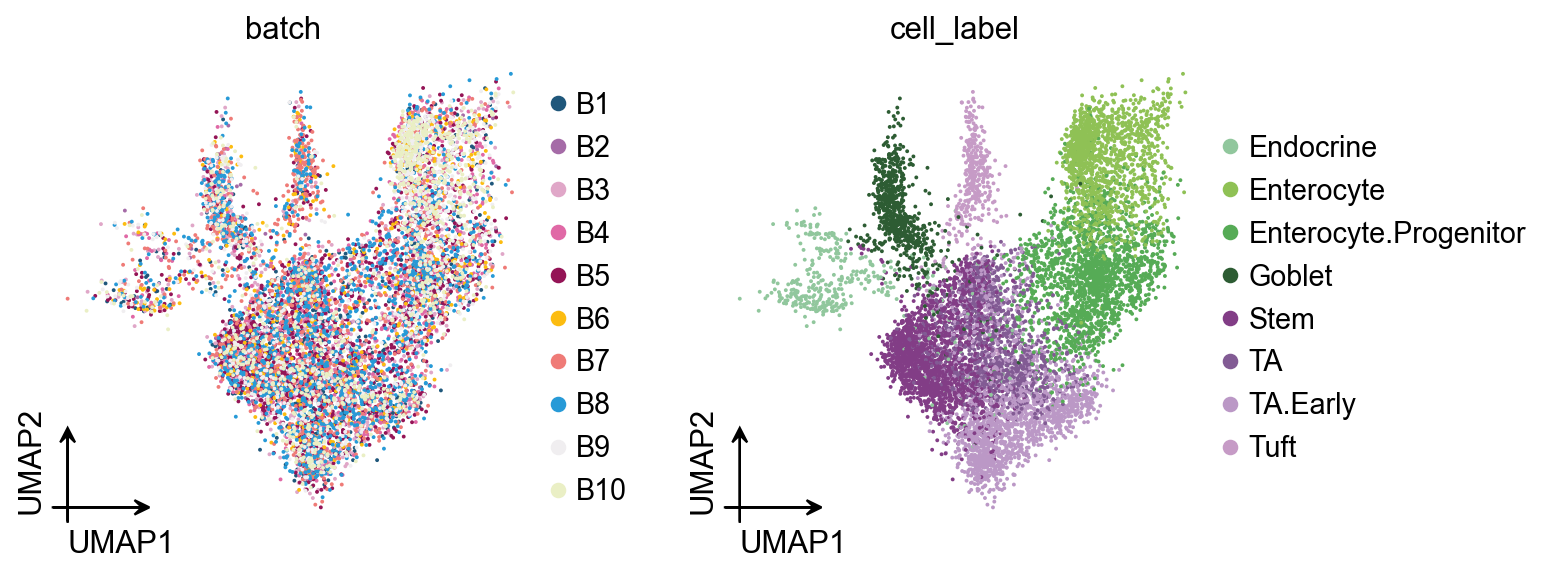
adata=ov.read('data/milo_test.h5ad')

ov.pl.umap(
    adata,
    color=['batch','cell_label'],
)

X_umap converted to UMAP to visualize and saved to adata.obsm['UMAP']
if you want to use X_umap, please set convert=False

Differential abundance testing with GLM

Similar to the scCODA approach, we use omicverse.single.DCT to perform differential cell–abundance analysis, except that here we set the method to milopy.

In releases after 1.7.9, we have removed the rpy2‐based edgeR dependency so that milo analyses can run entirely in a native Python environment. But we also keep the milo argument if user need the raw method

dct_obj=ov.single.DCT(
    adata,
    condition='condition',
    ctrl_group='Control',
    test_group='Salmonella',
    cell_type_key='cell_label',
    method='milopy',
    sample_key='batch',
    use_rep='X_harmony'
)

✅ Differential cell type abundance analysis initialized
📊 DCT analysis using milopy method
📊 Condition: condition, Control group: Control, Test group: Salmonella
computing neighbors
    finished: added to `.uns['neighbors']`
    `.obsp['distances']`, distances for each pair of neighbors
    `.obsp['connectivities']`, weighted adjacency matrix (0:00:21)

dct_obj.run()

✅ milopy DCT analysis completed

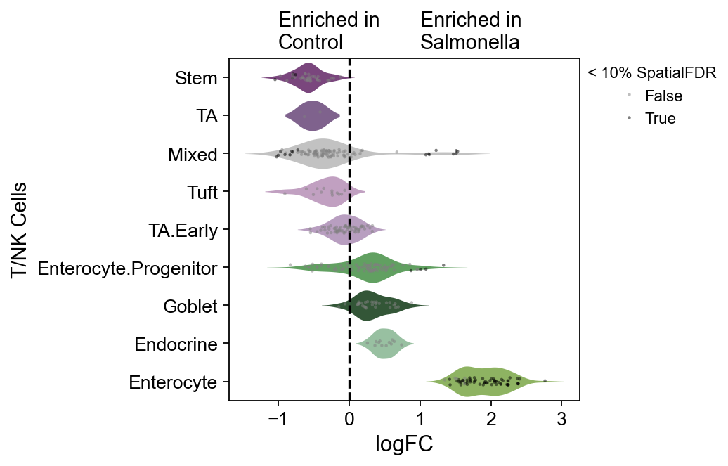
We can start inspecting the results of our DA analysis from a couple of standard diagnostic plots.

import matplotlib.pyplot as plt
old_figsize = plt.rcParams["figure.figsize"]
plt.rcParams["figure.figsize"] = [6, 3]
plt.subplot(1, 2, 1)
plt.hist(dct_obj.mdata["milo"].var.PValue, bins=50)
plt.xlabel("P-Vals")
plt.subplot(1, 2, 2)
plt.plot(dct_obj.mdata["milo"].var.logFC, -ov.np.log10(dct_obj.mdata["milo"].var.SpatialFDR), ".")
plt.xlabel("log-Fold Change")
plt.ylabel("- log10(Spatial FDR)")
plt.tight_layout()
plt.rcParams["figure.figsize"] = old_figsize

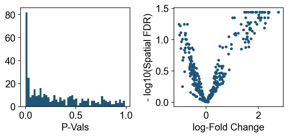
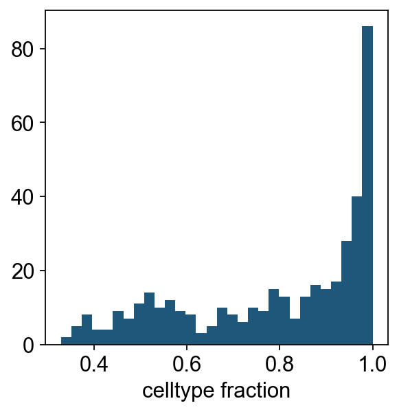
We can see that for the majority of neighbourhoods, almost all cells have the same cell type label. We can rename neighbourhoods where less than 60% of the cells have the top label as “Mixed”

plt.hist(dct_obj.mdata["milo"].var["nhood_annotation_frac"], bins=30)
plt.xlabel("celltype fraction")

Text(0.5, 0, 'celltype fraction')

res=dct_obj.get_results(mix_threshold=0.6)
res.head()

	index_cell	kth_distance	logFC	lfcSE	logCPM	stat	PValue	FDR	adj_pvalue	SpatialFDR	Nhood_size	nhood_annotation	nhood_annotation_frac
0	B1_AAACGCACTGTCCC_Control_Stem	9.152347	-0.583312	0.051568	11.412487	3.713398	0.080774	0.258990	0.258990	0.256133	399.0	Mixed	0.578947
1	B1_AATAAGCTAGAGAT_Control_Enterocyte.Progenitor	9.476911	-0.809424	0.056194	11.429808	8.896907	0.012736	0.079455	0.079455	0.079067	408.0	Mixed	0.524510
2	B1_ACGCTGCTCTCTTA_Control_Enterocyte.Progenitor	9.004735	1.512198	0.017016	10.817280	12.689494	0.004606	0.045980	0.045980	0.044634	228.0	Mixed	0.557018
3	B1_ACGGAACTGTTAGC_Control_Enterocyte.Progenitor	9.966439	0.673496	0.032412	10.452936	2.316397	0.156838	0.362072	0.362072	0.350619	181.0	Mixed	0.563536
4	B1_ACTTCTGATCGTTT_Control_TA.Early	9.194638	0.202095	0.035912	11.222971	0.404716	0.537956	0.714916	0.714916	0.705203	339.0	TA.Early	0.820059

Visualization

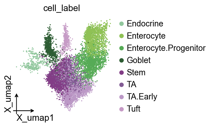
This is my favorite Milo plot. First, we create a color_dict to specify the cell colors we want to visualize.

color_dict=dict(zip(
    adata.obs['cell_label'].cat.categories,
    ov.pl.green_color[:4]+ov.pl.purple_color
))
color_dict['Mixed']='#c2c2c2'
fig, ax = plt.subplots(figsize=(3, 3))
ov.pl.embedding(
    adata,
    basis='X_umap',
    color=['cell_label'],
    palette=color_dict,
    ax=ax,
    #fig_size=(3,3)
)

#fig, ax = plt.subplots(figsize=(3, 4))
dct_obj.model.plot_da_beeswarm(
    dct_obj.mdata, 
    alpha=0.1,
    return_fig=True,
    palette=color_dict,
)
ov.plt.xticks(fontsize=12)
ov.plt.yticks(fontsize=12)
ov.plt.ylabel('T/NK Cells',fontsize=13)
ov.plt.text(-1,-0.75,'Enriched in\nControl',fontsize=13)
ov.plt.text(1,-0.75,'Enriched in\nSalmonella',fontsize=13)
#fig

Text(1, -0.75, 'Enriched in\nSalmonella')

(Optional) DCT with milo

Tutorials could be found in https://pertpy.readthedocs.io/en/stable/tutorials/notebooks/milo.html

dct_obj_old=ov.single.DCT(
    adata,
    condition='condition',
    ctrl_group='Control',
    test_group='Salmonella',
    cell_type_key='cell_label',
    method='milo',
    sample_key='batch',
    use_rep='X_harmony'
)

✅ Differential cell type abundance analysis initialized
📊 DCT analysis using milo method
📊 Condition: condition, Control group: Control, Test group: Salmonella
computing neighbors
    finished: added to `.uns['neighbors']`
    `.obsp['distances']`, distances for each pair of neighbors
    `.obsp['connectivities']`, weighted adjacency matrix (0:00:07)

dct_obj_old.run()

✅ milo DCT analysis completed

#fig, ax = plt.subplots(figsize=(3, 4))
dct_obj_old.model.plot_da_beeswarm(
    dct_obj_old.mdata, 
    alpha=0.1,
    return_fig=True,
    palette=color_dict,
)
ov.plt.xticks(fontsize=12)
ov.plt.yticks(fontsize=12)
ov.plt.ylabel('T/NK Cells',fontsize=13)
ov.plt.text(-1,-0.75,'Enriched in\nControl',fontsize=13)
ov.plt.text(1,-0.75,'Enriched in\nSalmonella',fontsize=13)
#fig

Text(1, -0.75, 'Enriched in\nSalmonella')