Trajectory Inference with StaVIA
VIA is a single-cell Trajectory Inference method that offers topology construction, pseudotimes, automated terminal state prediction and automated plotting of temporal gene dynamics along lineages. Here, we have improved the original author’s colouring logic and user habits so that users can use the anndata object directly for analysis。
We have completed this tutorial using the analysis provided by the original VIA authors.
Paper: Generalized and scalable trajectory inference in single-cell omics data with VIA
Code: https://github.com/ShobiStassen/VIA
Colab_Reproducibility:https://colab.research.google.com/drive/1A2X23z_RLJaYLbXaiCbZa-fjNbuGACrD?usp=sharing
import scanpy as sc
import omicverse as ov
from omicverse.external import VIA

import matplotlib.pyplot as plt
ov.plot_set()
   ____            _     _    __
  / __ \____ ___  (_)___| |  / /__  _____________
 / / / / __ `__ \/ / ___/ | / / _ \/ ___/ ___/ _ \
/ /_/ / / / / / / / /__ | |/ /  __/ /  (__  )  __/
\____/_/ /_/ /_/_/\___/ |___/\___/_/  /____/\___/

Version: 1.6.9, Tutorials: https://omicverse.readthedocs.io/
Dependency error: (pydeseq2 0.4.11 (/mnt/home/zehuazeng/software/rsc/lib/python3.10/site-packages), Requirement.parse('pydeseq2<=0.4.0,>=0.3'))
Preprocess data
As an example, we apply differential kinetic analysis to dentate gyrus neurogenesis, which comprises multiple heterogeneous subpopulations.
import scvelo as scv
adata=scv.datasets.dentategyrus()
adata
AnnData object with n_obs × n_vars = 2930 × 13913
    obs: 'clusters', 'age(days)', 'clusters_enlarged'
    uns: 'clusters_colors'
    obsm: 'X_umap'
    layers: 'ambiguous', 'spliced', 'unspliced'
adata=ov.pp.preprocess(adata,mode='shiftlog|pearson',n_HVGs=2000,)
adata.raw = adata
adata = adata[:, adata.var.highly_variable_features]
ov.pp.scale(adata)
ov.pp.pca(adata,layer='scaled',n_pcs=50)
Begin robust gene identification
After filtration, 13264/13913 genes are kept.     Among 13264 genes, 13189 genes are robust.
End of robust gene identification.
Begin size normalization: shiftlog and HVGs selection pearson
normalizing counts per cell. The following highly-expressed genes are not considered during normalization factor computation:
['Hba-a1', 'Malat1', 'Ptgds', 'Hbb-bt']
    finished (0:00:00)
extracting highly variable genes
--> added
    'highly_variable', boolean vector (adata.var)
    'highly_variable_rank', float vector (adata.var)
    'highly_variable_nbatches', int vector (adata.var)
    'highly_variable_intersection', boolean vector (adata.var)
    'means', float vector (adata.var)
    'variances', float vector (adata.var)
    'residual_variances', float vector (adata.var)
Time to analyze data in cpu: 1.2880923748016357 seconds.
End of size normalization: shiftlog and HVGs selection pearson
... as `zero_center=True`, sparse input is densified and may lead to large memory consumption
computing PCA
    with n_comps=50
    finished (0:00:00)
ov.pp.neighbors(adata,use_rep='scaled|original|X_pca',n_neighbors=15,n_pcs=30)
ov.pp.umap(adata,min_dist=1)
computing neighbors
    finished: added to `.uns['neighbors']`
    `.obsp['distances']`, distances for each pair of neighbors
    `.obsp['connectivities']`, weighted adjacency matrix (0:00:04)
computing UMAP
    finished: added
    'X_umap', UMAP coordinates (adata.obsm)
    'umap', UMAP parameters (adata.uns) (0:00:03)
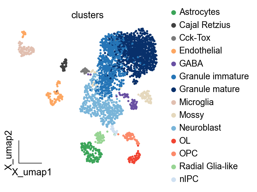
ov.pl.embedding(adata,basis='X_umap',
                   color=['clusters'],
                   frameon='small',cmap='Reds')
Model construct and run
We need to specify the cell feature vector use_rep used for VIA inference, which can be X_pca, X_scVI or X_glue, depending on the purpose of your analysis, here we use X_pca directly. We also need to specify how many components to be used, the components should not larger than the length of vector.
Besides, we need to specify the clusters to be colored and calculate for VIA. If the root_user is None, it will be calculated the root cell automatically.
We need to set basis argument stored in adata.obsm. An example setting tsne because it stored in obsm: 'tsne', 'MAGIC_imputed_data', 'palantir_branch_probs', 'X_pca'
We also need to set clusters argument stored in adata.obs. It means the celltype key.
Other explaination of argument and attributes could be found at https://pyvia.readthedocs.io/en/latest/notebooks/ViaJupyter_scRNA_Hematopoiesis.html
StaVia for time-series
StaVia for spatial-temporal
ncomps=30
knn=15
v0_random_seed=4
root_user = ['nIPC'] #the index of a cell belonging to the nIPC cell type
memory = 10
dataset = ''
use_rep = 'scaled|original|X_pca'
clusters = 'clusters'
basis='X_umap'

'''
#NOTE1, if you decide to choose a cell type as a root, then you need to set the dataset as 'group'
#root_user=['HSC1']
#dataset = 'group'# 'humanCD34'
#NOTE2, if rna-velocity is available, considering using it to compute the root automatically- see RNA velocity tutorial
'''

v0 = VIA.core.VIA(data=adata.obsm[use_rep][:, 0:ncomps],
             true_label=adata.obs[clusters],
             edgepruning_clustering_resolution=0.15, cluster_graph_pruning=0.15,
             knn=knn,  root_user=root_user, resolution_parameter=1.5,
             dataset=dataset, random_seed=v0_random_seed, memory=memory)#, do_compute_embedding=True, embedding_type='via-atlas')

v0.run_VIA()
Visualize and analysis
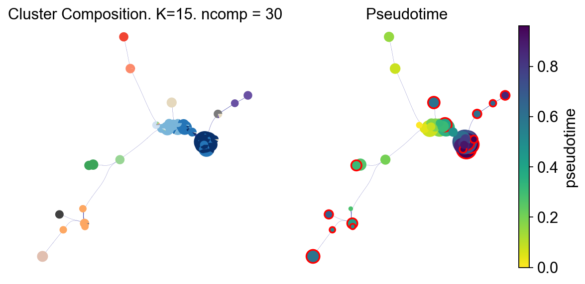
Before the subsequent analysis, we need to specify the colour of each cluster. Here we use sc.pl.embedding to automatically colour each cluster, if you need to specify your own colours, specify the palette parameter
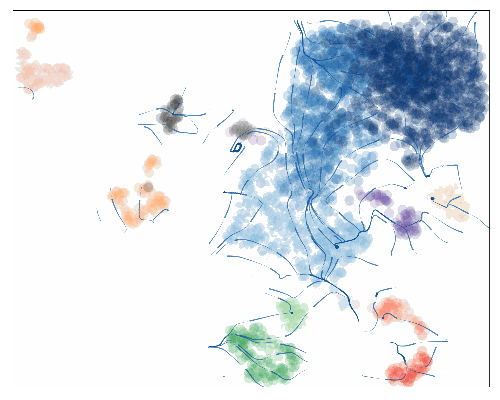
fig, ax, ax1 = VIA.core.plot_piechart_viagraph_ov(adata,clusters='clusters',dpi=80,
                                             via_object=v0, ax_text=False,show_legend=False)
fig.set_size_inches(8,4)
tune edges False
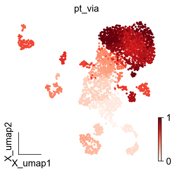
adata.obs['pt_via']=v0.single_cell_pt_markov
ov.pl.embedding(adata,basis='X_umap',
                   color=['pt_via'],
                   frameon='small',cmap='Reds')
Trajectory projection
Visualize the overall VIA trajectory projected onto a 2D embedding (UMAP, Phate, TSNE etc) in different ways.
Draw the high-level clustergraph abstraction onto the embedding;
Draw high-edge resolution directed graph
Draw a vector field/stream plot of the more fine-grained directionality of cells along the trajectory projected onto an embedding.
Key Parameters:
scatter_size
scatter_alpha
linewidth
draw_all_curves (if too crowded, set to False)
clusters='clusters'
color_true_list=adata.uns['{}_colors'.format(clusters)]
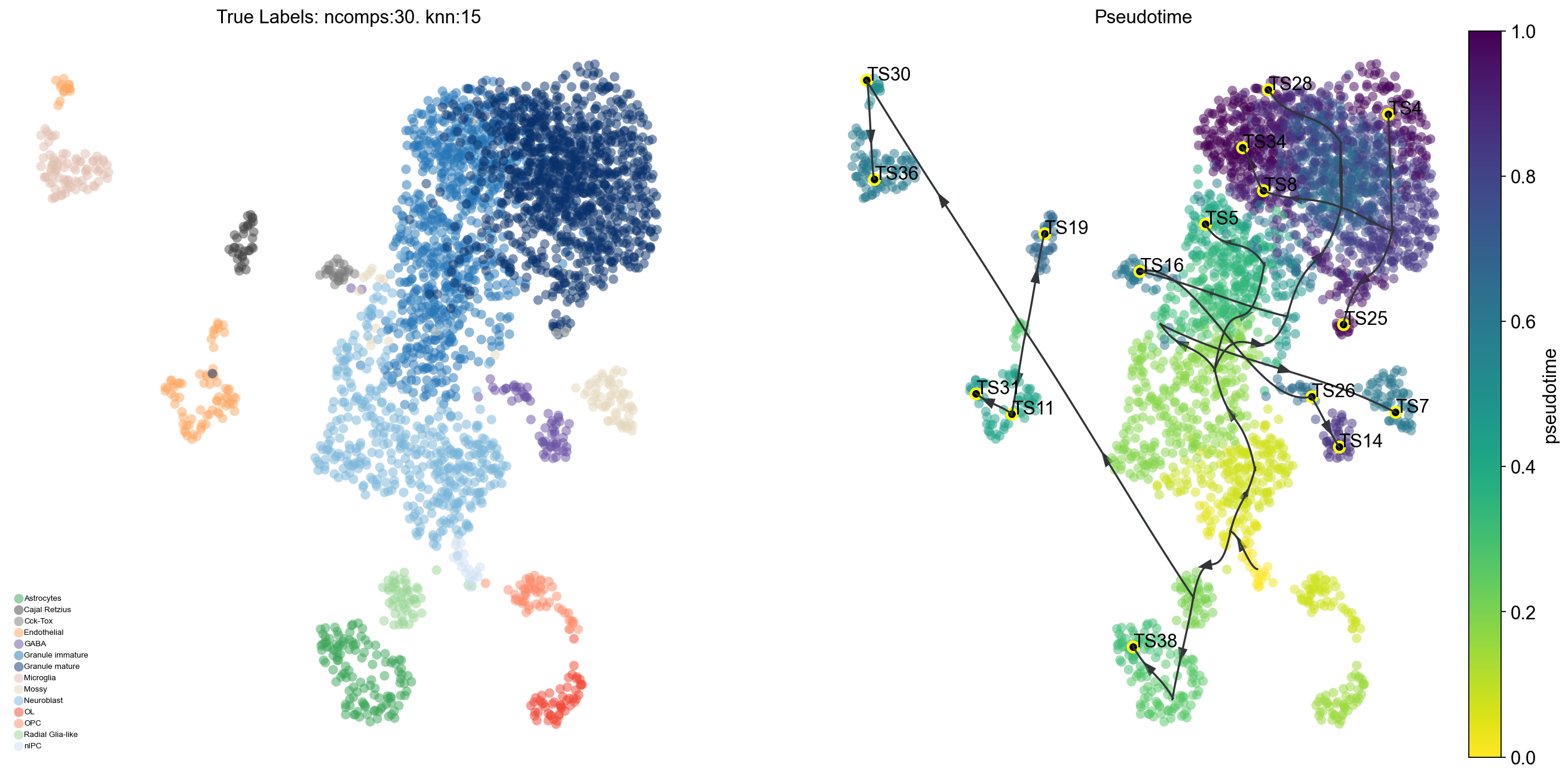
fig, ax, ax1 = VIA.core.plot_trajectory_curves_ov(adata,clusters='clusters',dpi=80,
                                                  via_object=v0,embedding=adata.obsm['X_umap'],
                                               draw_all_curves=False)
2024-12-17 21:32:16.116402	Super cluster 4 is a super terminal with sub_terminal cluster 34
2024-12-17 21:32:16.116705	Super cluster 5 is a super terminal with sub_terminal cluster 4
2024-12-17 21:32:16.116761	Super cluster 7 is a super terminal with sub_terminal cluster 5
2024-12-17 21:32:16.116808	Super cluster 8 is a super terminal with sub_terminal cluster 36
2024-12-17 21:32:16.116859	Super cluster 11 is a super terminal with sub_terminal cluster 7
2024-12-17 21:32:16.116910	Super cluster 14 is a super terminal with sub_terminal cluster 8
2024-12-17 21:32:16.117002	Super cluster 16 is a super terminal with sub_terminal cluster 38
2024-12-17 21:32:16.117057	Super cluster 19 is a super terminal with sub_terminal cluster 11
2024-12-17 21:32:16.117118	Super cluster 25 is a super terminal with sub_terminal cluster 14
2024-12-17 21:32:16.117166	Super cluster 26 is a super terminal with sub_terminal cluster 16
2024-12-17 21:32:16.117215	Super cluster 28 is a super terminal with sub_terminal cluster 19
2024-12-17 21:32:16.117263	Super cluster 30 is a super terminal with sub_terminal cluster 25
2024-12-17 21:32:16.117308	Super cluster 31 is a super terminal with sub_terminal cluster 26
2024-12-17 21:32:16.117360	Super cluster 34 is a super terminal with sub_terminal cluster 28
2024-12-17 21:32:16.117407	Super cluster 36 is a super terminal with sub_terminal cluster 30
2024-12-17 21:32:16.117453	Super cluster 38 is a super terminal with sub_terminal cluster 31
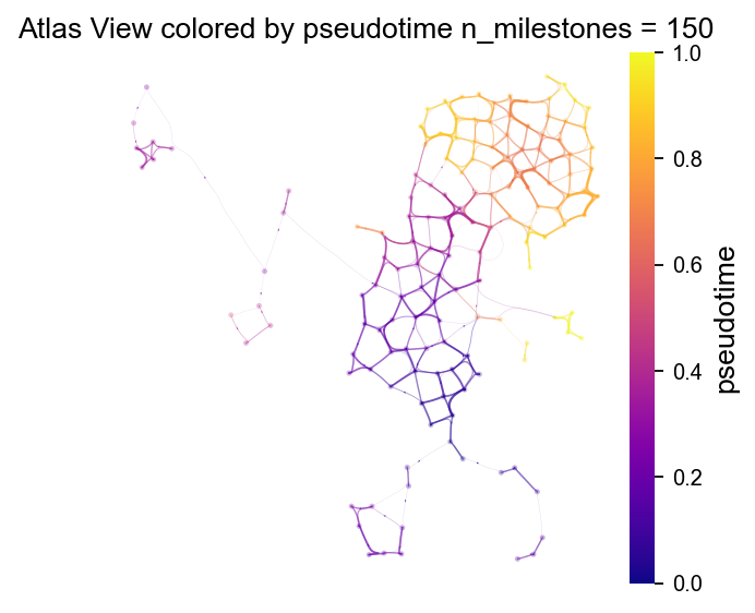
v0.embedding = adata.obsm['X_umap']
fig, ax = VIA.core.plot_atlas_view(via_object=v0,
                                   n_milestones=150,
                                   sc_labels=adata.obs['clusters'],
                                   fontsize_title=12,
                                   fontsize_labels=12,dpi=80,
                                   extra_title_text='Atlas View colored by pseudotime')
fig.set_size_inches(4,4)
2024-12-17 21:42:19.896260	Computing Edges
2024-12-17 21:42:19.896311	Start finding milestones
2024-12-17 21:42:20.368246	End milestones with 150
2024-12-17 21:42:20.371431	Recompute weights
2024-12-17 21:42:20.380990	pruning milestone graph based on recomputed weights
2024-12-17 21:42:20.381684	Graph has 1 connected components before pruning
2024-12-17 21:42:20.382195	Graph has 7 connected components after pruning
2024-12-17 21:42:20.386902	Graph has 1 connected components after reconnecting
2024-12-17 21:42:20.387577	regenerate igraph on pruned edges
2024-12-17 21:42:20.393241	Setting numeric label as time_series_labels or other sequential metadata for coloring edges
2024-12-17 21:42:20.401529	Making smooth edges
inside add sc embedding second if
# edge plots can be made with different edge resolutions. Run hammerbundle_milestone_dict() to recompute the edges for plotting. Then provide the new hammerbundle as a parameter to plot_edge_bundle()
# it is better to compute the edges and save them to the via_object. this gives more control to the merging of edges
decay = 0.6 #increasing decay increasing merging of edges
i_bw = 0.02 #increasing bw increases merging of edges
global_visual_pruning = 0.5 #higher number retains more edges
n_milestones = 200

v0.hammerbundle_milestone_dict= VIA.core.make_edgebundle_milestone(via_object=v0,
                                                              n_milestones=n_milestones,
                                                              decay=decay, initial_bandwidth=i_bw,
                                                              global_visual_pruning=global_visual_pruning)
2024-12-17 21:42:55.254801	Start finding milestones
2024-12-17 21:42:55.870327	End milestones with 200
2024-12-17 21:42:55.873729	Recompute weights
2024-12-17 21:42:55.886283	pruning milestone graph based on recomputed weights
2024-12-17 21:42:55.887059	Graph has 1 connected components before pruning
2024-12-17 21:42:55.887595	Graph has 5 connected components after pruning
2024-12-17 21:42:55.891122	Graph has 1 connected components after reconnecting
2024-12-17 21:42:55.891964	regenerate igraph on pruned edges
2024-12-17 21:42:55.898723	Setting numeric label as single cell pseudotime for coloring edges
2024-12-17 21:42:55.908959	Making smooth edges
fig, ax = VIA.core.plot_atlas_view(via_object=v0,
                              add_sc_embedding=True,
                              sc_labels_expression=adata.obs['clusters'],
                              cmap='jet', sc_labels=adata.obs['clusters'],
                              text_labels=True,
                              extra_title_text='Atlas View by Cell type',
                              fontsize_labels=3,fontsize_title=3,dpi=300
                             )
fig.set_size_inches(6,4)
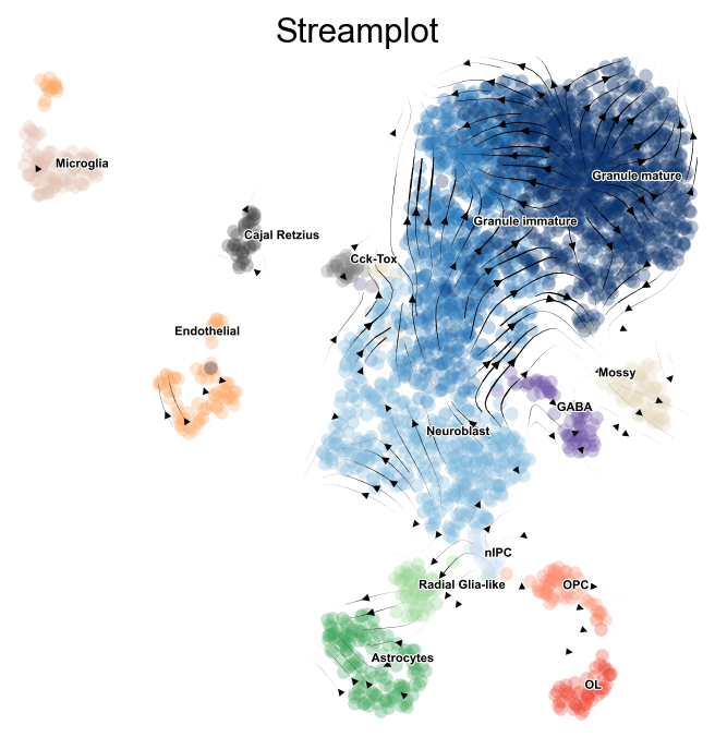
# via_streamplot() requires you to either provide an ndarray as embedding as an input parameter OR for via to have an embedding attribute
fig, ax = VIA.core.via_streamplot_ov(adata,'clusters',
                                     v0, embedding=adata.obsm['X_umap'], dpi=80,
                             density_grid=0.8, scatter_size=30,
                             scatter_alpha=0.3, linewidth=0.5)
fig.set_size_inches(5,5)
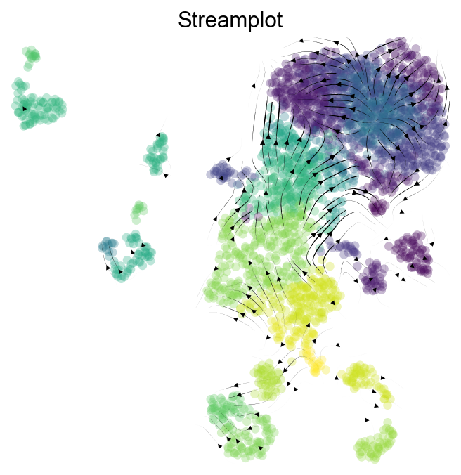
#Colored by pseudotime

fig, ax = VIA.core.via_streamplot_ov(adata,'clusters',
                             v0,density_grid=0.8, scatter_size=30, color_scheme='time', linewidth=0.5,
                             min_mass = 1, cutoff_perc = 5, scatter_alpha=0.3, marker_edgewidth=0.1,
                             density_stream = 2, smooth_transition=1, smooth_grid=0.5,dpi=80,)
fig.set_size_inches(5,5)
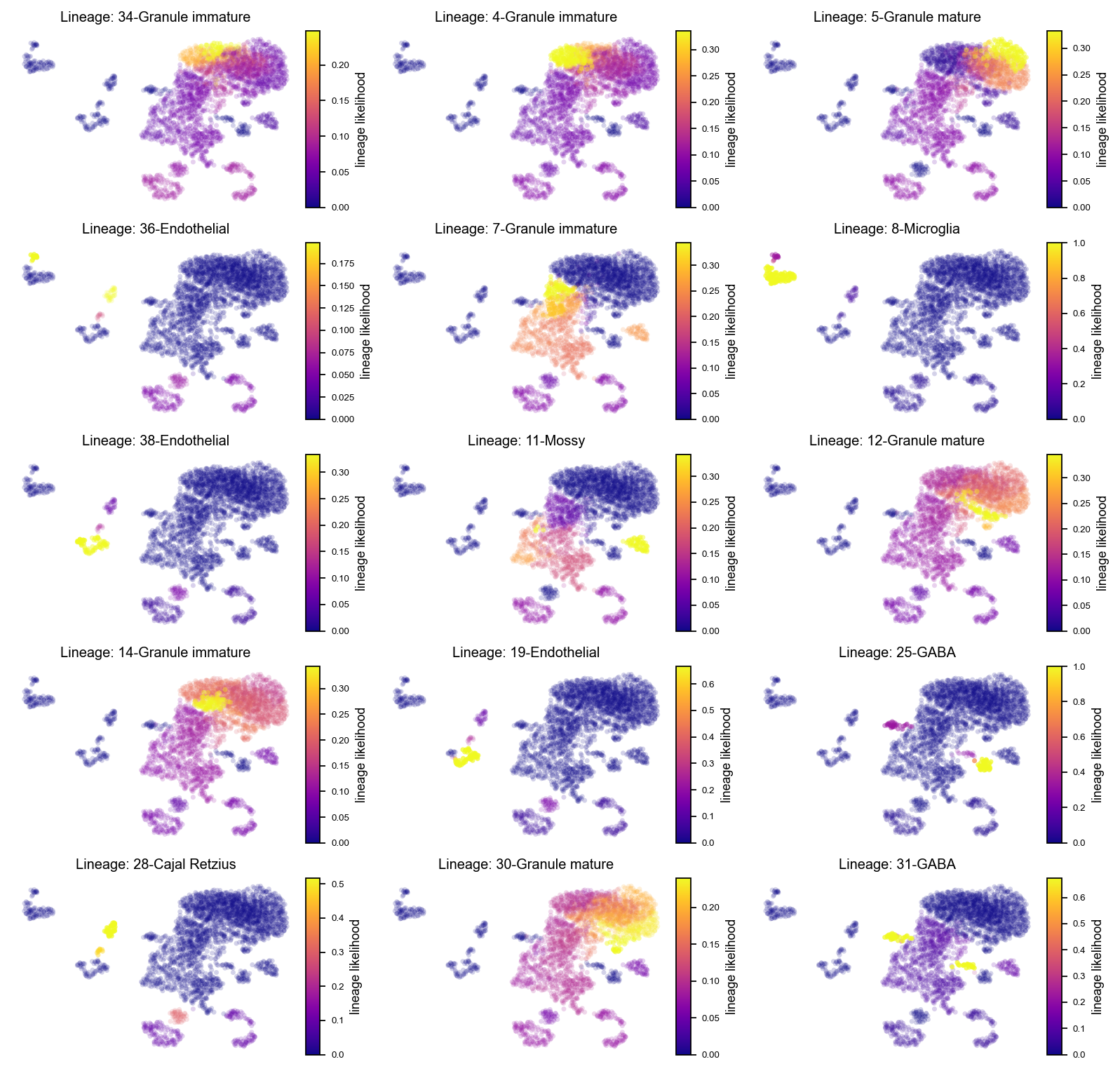
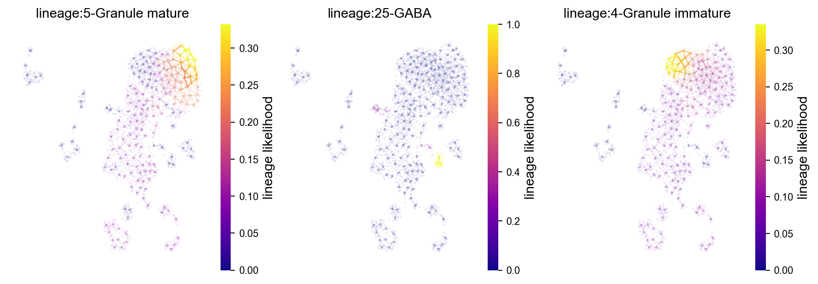
Probabilistic pathways and Memory
Visualize the probabilistic pathways from root to terminal state as indicated by the lineage likelihood. The higher the linage likelihood, the greater the potential of that particular cell to differentiate towards the terminal state of interest. Changing the memory paramater will alter the specificity of the lineage pathway. This can be visualized at the single-cell level but also combined with the Atlas View which visualizes cell-cell connectivity and pathways
Key Parameters:
marker_lineages (list) of terminal clusters
fig, axs= VIA.core.plot_sc_lineage_probability(via_object=v0, dpi=80,
                                          #marker_lineages=[7,11,12,15,20,22],
                                          embedding=adata.obsm['X_umap']) #marker_lineages=v0.terminal_clusters to plot all
fig.set_size_inches(12,12)
2024-12-17 21:48:09.698594	Marker_lineages: [34, 4, 5, 36, 7, 8, 38, 11, 12, 14, 19, 25, 28, 30, 31]
2024-12-17 21:48:09.700021	The number of components in the original full graph is 1
2024-12-17 21:48:09.700039	For downstream visualization purposes we are also constructing a low knn-graph
2024-12-17 21:48:13.845602	Check sc pb 1.0
f getting majority comp
2024-12-17 21:48:13.875623	Cluster path on clustergraph starting from Root Cluster 33 to Terminal Cluster 34: [33, 23, 2, 1, 3, 24, 18, 37, 6, 34]
2024-12-17 21:48:13.875656	Cluster path on clustergraph starting from Root Cluster 33 to Terminal Cluster 4: [33, 23, 2, 1, 3, 24, 18, 37, 6, 22, 4]
2024-12-17 21:48:13.875677	Cluster path on clustergraph starting from Root Cluster 33 to Terminal Cluster 5: [33, 23, 2, 1, 3, 24, 18, 37, 6, 5]
2024-12-17 21:48:13.875696	Cluster path on clustergraph starting from Root Cluster 33 to Terminal Cluster 36: [33, 23, 21, 40, 36]
2024-12-17 21:48:13.875718	Cluster path on clustergraph starting from Root Cluster 33 to Terminal Cluster 7: [33, 23, 2, 1, 3, 7]
2024-12-17 21:48:13.875737	Cluster path on clustergraph starting from Root Cluster 33 to Terminal Cluster 8: [33, 23, 21, 40, 36, 8]
2024-12-17 21:48:13.875755	Cluster path on clustergraph starting from Root Cluster 33 to Terminal Cluster 38: [33, 23, 21, 40, 19, 38]
2024-12-17 21:48:13.875773	Cluster path on clustergraph starting from Root Cluster 33 to Terminal Cluster 11: [33, 23, 27, 9, 29, 11]
2024-12-17 21:48:13.875792	Cluster path on clustergraph starting from Root Cluster 33 to Terminal Cluster 12: [33, 23, 2, 1, 3, 24, 18, 35, 12]
2024-12-17 21:48:13.875811	Cluster path on clustergraph starting from Root Cluster 33 to Terminal Cluster 14: [33, 23, 2, 1, 3, 24, 18, 35, 14]
2024-12-17 21:48:13.875829	Cluster path on clustergraph starting from Root Cluster 33 to Terminal Cluster 19: [33, 23, 21, 40, 19]
2024-12-17 21:48:13.875848	Cluster path on clustergraph starting from Root Cluster 33 to Terminal Cluster 25: [33, 23, 2, 1, 3, 24, 26, 31, 25]
2024-12-17 21:48:13.875866	Cluster path on clustergraph starting from Root Cluster 33 to Terminal Cluster 28: [33, 23, 21, 40, 28]
2024-12-17 21:48:13.875885	Cluster path on clustergraph starting from Root Cluster 33 to Terminal Cluster 30: [33, 23, 2, 1, 3, 24, 18, 35, 12, 30]
2024-12-17 21:48:13.875904	Cluster path on clustergraph starting from Root Cluster 33 to Terminal Cluster 31: [33, 23, 2, 1, 3, 24, 26, 31]
setting vmin to 0.0
2024-12-17 21:48:14.002431	Revised Cluster level path on sc-knnGraph from Root Cluster 33 to Terminal Cluster 34 along path: [33, 33, 29, 7, 4, 34]
setting vmin to 0.0
2024-12-17 21:48:14.019380	Revised Cluster level path on sc-knnGraph from Root Cluster 33 to Terminal Cluster 4 along path: [33, 33, 29, 7, 4, 4, 4]
setting vmin to 0.0
2024-12-17 21:48:14.036054	Revised Cluster level path on sc-knnGraph from Root Cluster 33 to Terminal Cluster 5 along path: [33, 33, 29, 22, 5, 5]
setting vmin to 0.0
2024-12-17 21:48:14.053328	Revised Cluster level path on sc-knnGraph from Root Cluster 33 to Terminal Cluster 36 along path: [33, 33, 23, 40, 36, 36]
setting vmin to 0.0
2024-12-17 21:48:14.070809	Revised Cluster level path on sc-knnGraph from Root Cluster 33 to Terminal Cluster 7 along path: [33, 33, 29, 3, 13, 7, 7]
setting vmin to 0.0
2024-12-17 21:48:14.087681	Revised Cluster level path on sc-knnGraph from Root Cluster 33 to Terminal Cluster 8 along path: [33, 33, 23, 40, 36, 8, 8, 8]
setting vmin to 0.0
2024-12-17 21:48:14.104397	Revised Cluster level path on sc-knnGraph from Root Cluster 33 to Terminal Cluster 38 along path: [33, 33, 23, 40, 19, 38, 38]
setting vmin to 0.0
2024-12-17 21:48:14.121445	Revised Cluster level path on sc-knnGraph from Root Cluster 33 to Terminal Cluster 11 along path: [33, 33, 1, 11, 11, 11]
setting vmin to 0.0
2024-12-17 21:48:14.138692	Revised Cluster level path on sc-knnGraph from Root Cluster 33 to Terminal Cluster 12 along path: [33, 33, 1, 26, 12, 12]
setting vmin to 0.0
2024-12-17 21:48:14.155534	Revised Cluster level path on sc-knnGraph from Root Cluster 33 to Terminal Cluster 14 along path: [33, 33, 23, 40, 18, 14, 14]
setting vmin to 0.0
2024-12-17 21:48:14.171974	Revised Cluster level path on sc-knnGraph from Root Cluster 33 to Terminal Cluster 19 along path: [33, 33, 23, 40, 19, 19]
setting vmin to 0.0
2024-12-17 21:48:14.188618	Revised Cluster level path on sc-knnGraph from Root Cluster 33 to Terminal Cluster 25 along path: [33, 33, 1, 31, 26, 25, 25, 25]
setting vmin to 0.0
2024-12-17 21:48:14.205329	Revised Cluster level path on sc-knnGraph from Root Cluster 33 to Terminal Cluster 28 along path: [33, 33, 23, 2, 28, 28, 28]
setting vmin to 0.0
2024-12-17 21:48:14.221767	Revised Cluster level path on sc-knnGraph from Root Cluster 33 to Terminal Cluster 30 along path: [33, 33, 1, 26, 30, 30, 30]
setting vmin to 0.0
2024-12-17 21:48:14.238223	Revised Cluster level path on sc-knnGraph from Root Cluster 33 to Terminal Cluster 31 along path: [33, 33, 1, 31, 31, 31]
fig, axs= VIA.core.plot_atlas_view(via_object=v0, dpi=80,
                              lineage_pathway=[5,25,4],
                                   fontsize_title = 12,
                                 fontsize_labels = 12,
                             ) #marker_lineages=v0.terminal_clusters to plot all
fig.set_size_inches(12,4)
location of 5 is at [2] and 2
setting vmin to 0.0
location of 25 is at [11] and 11
setting vmin to 0.0
location of 4 is at [1] and 1
setting vmin to 0.0
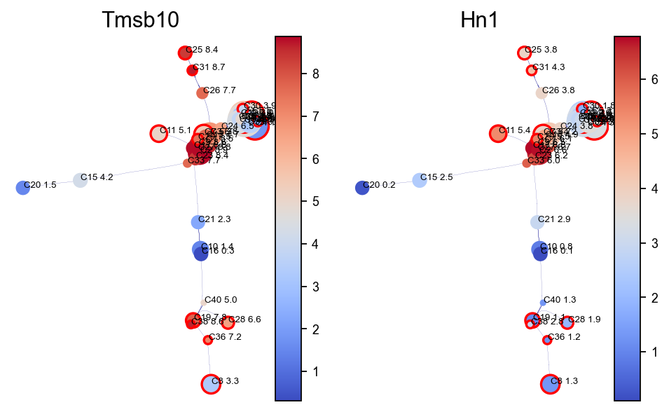
Visualise gene/feature graph
View the gene expression along the VIA graph. We use the computed HNSW small world graph in VIA to accelerate the gene imputation calculations (using similar approach to MAGIC) as follows:
import pandas as pd
gene_list_magic =['Tmsb10', 'Hn1', ]
df = adata.to_df()
df_magic = v0.do_impute(df, magic_steps=3, gene_list=gene_list_magic) #optional
shape of transition matrix raised to power 3 (2930, 2930)
fig, axs = VIA.core.plot_viagraph(via_object=v0,
                                  type_data='gene',
                                  df_genes=df_magic,
                                  gene_list=gene_list_magic[0:3], arrow_head=0.1)
fig.set_size_inches(12,4)
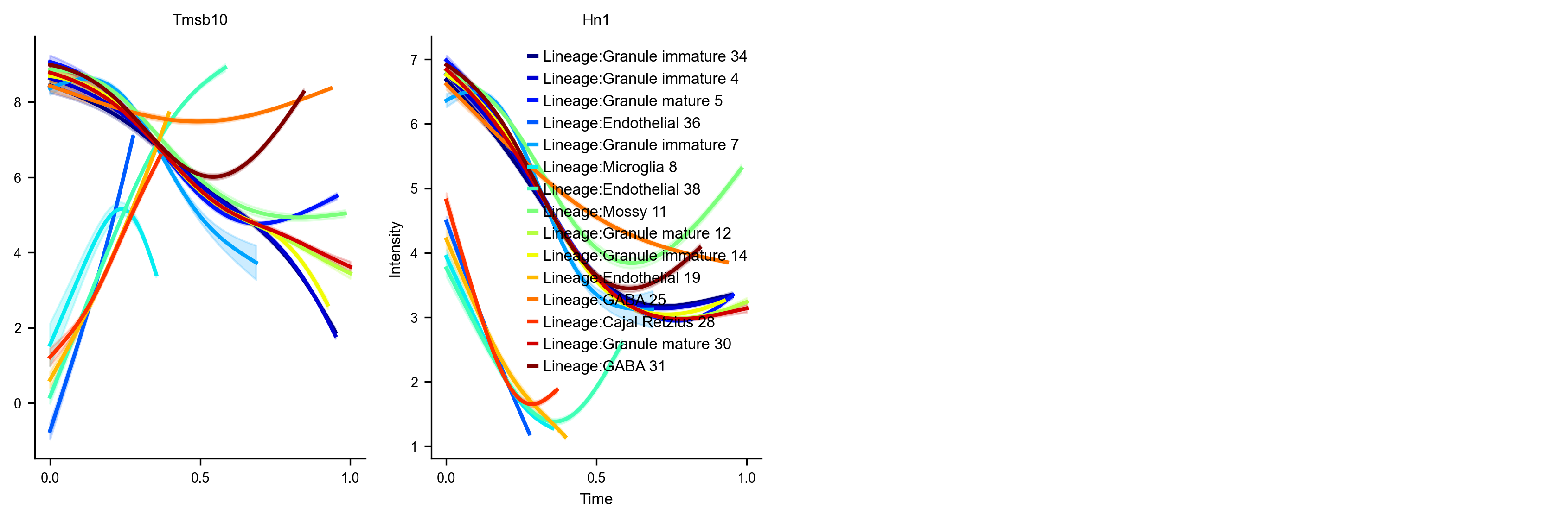
Gene Dynamics
The gene dynamics along pseudotime for all detected lineages are automatically inferred by VIA. These can be interpreted as the change in gene expression along any given lineage.
Key Parameters
n_splines
spline_order
gene_exp (dataframe) single-cell level gene expression of select genes (gene imputation is an optional pre-step)
fig, axs=VIA.core.get_gene_expression(via_object=v0, #cmap_dict=color_dict,
                                      gene_exp=df_magic[gene_list_magic])
fig.set_size_inches(14,4)
shape of transition matrix raised to power 3 (2930, 2930)
Area under curve Tmsb10 for branch Granule immature is 5.580818079102432
Area under curve Tmsb10 for branch Granule immature is 5.6305885516322896
Area under curve Tmsb10 for branch Granule mature is 6.09801291248822
Area under curve Tmsb10 for branch Endothelial is 0.8029748380565134
Area under curve Tmsb10 for branch Granule immature is 4.553506054484809
Area under curve Tmsb10 for branch Microglia is 1.394565066745735
Area under curve Tmsb10 for branch Endothelial is 3.151271164024714
Area under curve Tmsb10 for branch Mossy is 6.381610292676225
Area under curve Tmsb10 for branch Granule mature is 6.013508411025893
Area under curve Tmsb10 for branch Granule immature is 5.664759428181174
Area under curve Tmsb10 for branch Endothelial is 1.5305425977544975
Area under curve Tmsb10 for branch GABA is 7.320013684508645
Area under curve Tmsb10 for branch Cajal Retzius is 1.3306728398525145
Area under curve Tmsb10 for branch Granule mature is 6.038859274125032
Area under curve Tmsb10 for branch GABA is 6.166411645842841
Area under curve Hn1 for branch Granule immature is 4.080599759640161
Area under curve Hn1 for branch Granule immature is 4.099823609762209
Area under curve Hn1 for branch Granule mature is 4.122596472992743
Area under curve Hn1 for branch Endothelial is 0.7689116578065938
Area under curve Hn1 for branch Granule immature is 3.2573533211918653
Area under curve Hn1 for branch Microglia is 0.8290642227866547
Area under curve Hn1 for branch Endothelial is 1.2344735137134157
Area under curve Hn1 for branch Mossy is 4.869794880657756
Area under curve Hn1 for branch Granule mature is 4.233111600633526
Area under curve Hn1 for branch Granule immature is 4.008845163737272
Area under curve Hn1 for branch Endothelial is 0.9515090694728756
Area under curve Hn1 for branch GABA is 4.5523504696409685
Area under curve Hn1 for branch Cajal Retzius is 0.9522895574200774
Area under curve Hn1 for branch Granule mature is 4.220430019708672
Area under curve Hn1 for branch GABA is 3.951854977018495
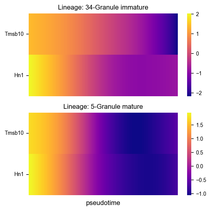
fig, axs = VIA.core.plot_gene_trend_heatmaps(via_object=v0,
                                             df_gene_exp=df_magic, cmap='plasma',
                                         marker_lineages=[34,5])
fig.set_size_inches(5,5)
branches [34, 5]
VIA.core.animate_streamplot_ov(adata,'clusters',v0, embedding=adata.obsm['X_umap'],
                       cmap_stream='Blues',
                       scatter_size=200, scatter_alpha=0.2, marker_edgewidth=0.15,
                        density_grid=0.7, linewidth=0.1,
                       segment_length=1.5,
                       saveto='result/animation_test.gif')
from IPython.display import Image

with open('result/animation_test.gif','rb') as file:
    display(Image(file.read(),width=400,height=400))
VIA.core.animate_atlas(via_object=v0,
                        extra_title_text='test animation',
                        n_milestones=None,
                        saveto='result/edgebundle_test.gif')
from IPython.display import Image

with open('result/edgebundle_test.gif','rb') as file:
    display(Image(file.read(),width=500,height=500))