Different Expression Analysis

An important task of bulk rna-seq analysis is the different expression , which we can perform with omicverse. For different expression analysis, ov change the gene_id to gene_name of matrix first. When our dataset existed the batch effect, we can use the SizeFactors of DEseq2 to normalize it, and use t-test of wilcoxon to calculate the p-value of genes. Here we demonstrate this pipeline with a matrix from featureCounts. The same pipeline would generally be used to analyze any collection of RNA-seq tasks.

Colab_Reproducibility：https://colab.research.google.com/drive/1q5lDfJepbtvNtc1TKz-h4wGUifTZ3i0_?usp=sharing

import omicverse as ov
import scanpy as sc
import matplotlib.pyplot as plt

ov.plot_set()

Warning: Could not read dependencies from pyproject.toml: [Errno 2] No such file or directory: '/home/groups/xiaojie/steorra/env/omicverse/lib/python3.10/site-packages/omicverse/pyproject.toml'

   ____            _     _    __                  
  / __ \____ ___  (_)___| |  / /__  _____________ 
 / / / / __ `__ \/ / ___/ | / / _ \/ ___/ ___/ _ \ 
/ /_/ / / / / / / / /__ | |/ /  __/ /  (__  )  __/ 
\____/_/ /_/ /_/_/\___/ |___/\___/_/  /____/\___/                                              

Version: 1.6.11, Tutorials: https://omicverse.readthedocs.io/

Geneset Download

When we need to convert a gene id, we need to prepare a mapping pair file. Here we have pre-processed 6 genome gtf files and generated mapping pairs including T2T-CHM13, GRCh38, GRCh37, GRCm39, danRer7, and danRer11. If you need to convert other id_mapping, you can generate your own mapping using gtf Place the files in the genesets directory.

ov.utils.download_geneid_annotation_pair()

......Geneid Annotation Pair download start: pair_GRCm39
......Loading dataset from genesets/pair_GRCm39.tsv
......Geneid Annotation Pair download start: pair_T2TCHM13
......Loading dataset from genesets/pair_T2TCHM13.tsv
......Geneid Annotation Pair download start: pair_GRCh38
......Loading dataset from genesets/pair_GRCh38.tsv
......Geneid Annotation Pair download start: pair_GRCh37
......Loading dataset from genesets/pair_GRCh37.tsv
......Geneid Annotation Pair download start: pair_danRer11
......Loading dataset from genesets/pair_danRer11.tsv
......Geneid Annotation Pair download start: pair_danRer7
......Loading dataset from genesets/pair_danRer7.tsv
......Geneid Annotation Pair download finished!

Note that this dataset has not been processed in any way and is only exported by featureCounts, and Sequence alignment was performed from the genome file of CRCm39

sample data can be download from: https://raw.githubusercontent.com/Starlitnightly/omicverse/master/sample/counts.txt

data=ov.pd.read_csv('https://raw.githubusercontent.com/Starlitnightly/omicverse/master/sample/counts.txt',index_col=0,sep='\t',header=1)
#data=ov.read('data/counts.txt',index_col=0,header=1)
#replace the columns `.bam` to `` 
data.columns=[i.split('/')[-1].replace('.bam','') for i in data.columns]
data.head()

	1--1	1--2	2--1	2--2	3--1	3--2	4--1	4--2	4-3	4-4	Blank-1	Blank-2
Geneid
ENSMUSG00000102628	0	0	0	0	5	0	0	0	0	0	0	9
ENSMUSG00000100595	0	0	0	0	0	0	0	0	0	0	0	0
ENSMUSG00000097426	5	0	0	0	0	0	0	1	0	0	0	0
ENSMUSG00000104478	0	0	0	0	0	0	0	0	0	0	0	0
ENSMUSG00000104385	0	0	0	0	0	0	0	0	0	0	0	0

ID mapping

We performed the gene_id mapping by the mapping pair file GRCm39 downloaded before.

data=ov.bulk.Matrix_ID_mapping(data,'genesets/pair_GRCm39.tsv')
data.head()

	1--1	1--2	2--1	2--2	3--1	3--2	4--1	4--2	4-3	4-4	Blank-1	Blank-2
Gm37732	0	0	0	0	0	0	0	0	0	0	0	0
ENSMUSG00002075679	0	0	0	0	0	0	0	0	0	0	0	0
Mir485	0	0	0	0	0	0	0	0	0	0	0	0
Gm45619	6	1	6	3	3	9	4	2	22	3	0	17
Gm25097	0	0	0	0	0	0	0	0	0	0	0	0

Different expression analysis with ov

We can do differential expression analysis very simply by ov, simply by providing an expression matrix. To run DEG, we simply need to:

• Read the raw count by featureCount or any other qualify methods.

• Create an ov DEseq object.

dds=ov.bulk.pyDEG(data)

We notes that the gene_name mapping before exist some duplicates, we will process the duplicate indexes to retain only the highest expressed genes

dds.drop_duplicates_index()
print('... drop_duplicates_index success')

... drop_duplicates_index success

We also need to remove the batch effect of the expression matrix, estimateSizeFactors of DEseq2 to be used to normalize our matrix

dds.normalize()
print('... estimateSizeFactors and normalize success')

... estimateSizeFactors and normalize success

Now we can calculate the different expression gene from matrix, we need to input the treatment and control groups

ttest

treatment_groups=['4-3','4-4']
control_groups=['1--1','1--2']
result_ttest=dds.deg_analysis(treatment_groups,control_groups,method='ttest')
result_ttest.sort_values('qvalue').head()

⚙️ You are using ttest method for differential expression analysis.
⏰ Start to calculate qvalue...
✅ Differential expression analysis completed.

	pvalue	qvalue	FoldChange	MaxBaseMean	BaseMean	log2(BaseMean)	log2FC	abs(log2FC)	size	-log(pvalue)	-log(qvalue)	sig
gene_id
Uqcrh	0.000005	0.000009	1.340669	2847.780642	2485.934617	11.279573	0.422953	0.422953	0.134067	5.341574	5.050298	sig
Tdrd7	0.000016	0.000031	0.819932	570.613422	519.217650	9.020196	-0.286423	0.286423	0.081993	4.796963	4.505703	sig
Glo1-ps	0.000016	0.000032	0.538839	1718.087949	1321.875745	10.368371	-0.892074	0.892074	0.053884	4.792256	4.501011	sig
Kmt2a	0.000023	0.000045	1.203046	1337.209316	1224.344556	10.257794	0.266692	0.266692	0.120305	4.638583	4.347354	sig
5730522E02Rik	0.000028	0.000054	34.728018	7.971628	3.985814	1.994874	5.118028	5.118028	3.472802	4.560393	4.270316	sig

(optional) edgeR with python

This module is a partial port in Python of the R Bioconductor edgeR package.

result_edgepy=dds.deg_analysis(treatment_groups,control_groups,method='edgepy')
result_edgepy.sort_values('qvalue').head()

⚙️ You are using edgepy method for differential expression analysis.
⏰ Start to create DGEList...
⏰ Start to calculate qvalue...
✅ Differential expression analysis completed.

	pvalue	qvalue	FoldChange	MaxBaseMean	BaseMean	log2(BaseMean)	log2FC	abs(log2FC)	size	-log(pvalue)	-log(qvalue)	sig
gene_id
Krtap9-5	2.904895e-46	1.583284e-41	0.000473	1547.775572	774.135593	9.596442	-11.046357	11.046357	1.104636	45.536870	40.800441	sig
Krtap31-2	2.824260e-36	7.696673e-32	0.005276	2119.945065	1065.447800	10.057244	-7.566236	7.566236	0.756624	35.549095	31.113697	sig
Krtap19-4	7.394568e-34	1.343445e-29	0.007051	1801.648929	907.058833	9.825052	-7.147957	7.147957	0.714796	33.131087	28.871780	sig
Gm4553	2.906425e-33	3.960294e-29	0.007580	1747.474564	880.242980	9.781758	-7.043576	7.043576	0.704358	32.536641	28.402273	sig
Gm10153	1.665008e-29	1.512493e-25	0.000884	267.271967	133.635984	7.062165	-10.144441	10.144441	1.014444	28.778584	24.820307	sig

(optional) limma

This module is a partial port in Python of the R Bioconductor limma package.

result_limma=dds.deg_analysis(treatment_groups,control_groups,method='limma')
result_limma.sort_values('qvalue').head()

⚙️ You are using limma method for differential expression analysis.
⏰ Start to create DGEList...
⏰ Start to adjust pvalue...
✅ Differential expression analysis completed.

	pvalue	qvalue	FoldChange	MaxBaseMean	BaseMean	log2(BaseMean)	log2FC	abs(log2FC)	size	sig	-log(pvalue)	-log(qvalue)	F	t
gene_id
Gm5853	0.000011	0.007723	5.216002	0.996454	0.498227	-1.005126	2.382945	2.382945	0.238294	sig	4.951007	2.112206	31871.910979	178.527060
Gm14409	0.000011	0.007723	5.216002	0.996454	0.498227	-1.005126	2.382945	2.382945	0.238294	sig	4.951007	2.112206	31871.910979	178.527060
Tdrd7	0.000005	0.007723	0.819932	570.613422	519.217650	9.020196	-0.286423	0.286423	0.028642	sig	5.330687	2.112206	69832.580356	-264.258548
Myl10	0.000009	0.007723	13.648007	2.989361	1.494680	0.579837	3.770618	3.770618	0.377062	sig	5.052672	2.112206	39320.908935	198.295005
5730522E02Rik	0.000009	0.007723	34.728018	7.971628	3.985814	1.994874	5.118028	5.118028	0.511803	sig	5.064980	2.112206	40333.534198	200.832105

One important thing is that we do not filter out low expression genes when processing DEGs, and in future versions I will consider building in the corresponding processing.

print(dds.result.shape)
dds.result=dds.result.loc[dds.result['log2(BaseMean)']>1]
print(dds.result.shape)

(54504, 14)
(21279, 14)

We also need to set the threshold of Foldchange, we prepare a method named foldchange_set to finish. This function automatically calculates the appropriate threshold based on the log2FC distribution, but you can also enter it manually.

# -1 means automatically calculates
dds.foldchange_set(fc_threshold=-1,
                   pval_threshold=0.05,
                   logp_max=6)

... Fold change threshold: 1.569942639522294

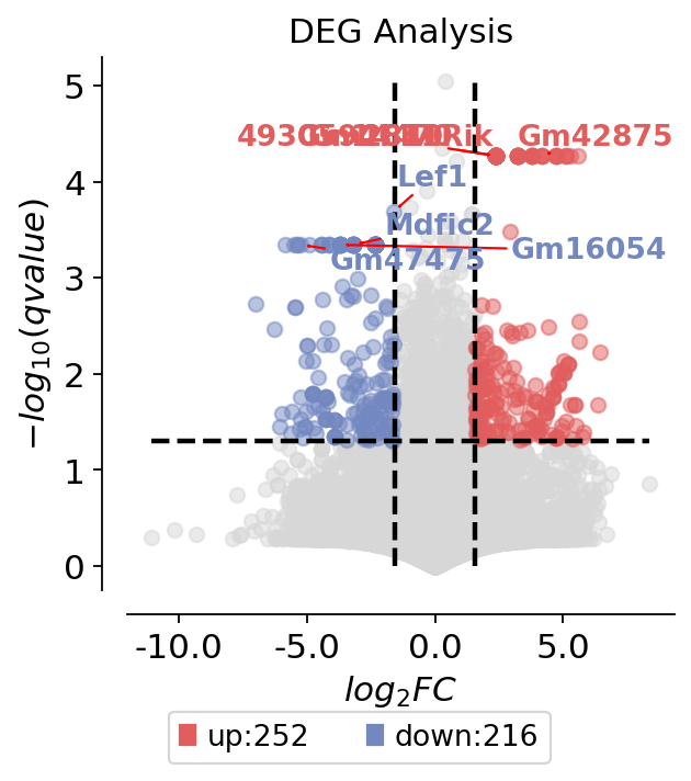
Visualize the DEG result and specific genes

To visualize the DEG result, we use plot_volcano to do it. This fuction can visualize the gene interested or high different expression genes. There are some parameters you need to input:

• title: The title of volcano

• figsize: The size of figure

• plot_genes: The genes you interested

• plot_genes_num: If you don’t have interested genes, you can auto plot it.

dds.plot_volcano(title='DEG Analysis',figsize=(4,4),
                 plot_genes_num=8,plot_genes_fontsize=12,)

<AxesSubplot: title={'center': 'DEG Analysis'}, xlabel='$log_{2}FC$', ylabel='$-log_{10}(qvalue)$'>

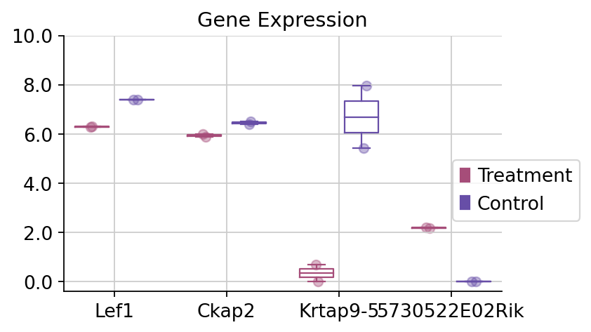
To visualize the specific genes, we only need to use the dds.plot_boxplot function to finish it.

dds.plot_boxplot(genes=['Ckap2','Lef1','Krtap9-5','5730522E02Rik'],treatment_groups=treatment_groups,
                control_groups=control_groups,figsize=(5,3),fontsize=12,
                 legend_bbox=(1.2,0.55))

(<Figure size 400x240 with 1 Axes>,
 <AxesSubplot: title={'center': 'Gene Expression'}>)

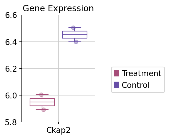
fig,ax=dds.plot_boxplot(genes=['Ckap2'],treatment_groups=treatment_groups,
                control_groups=control_groups,figsize=(2,3),fontsize=12,
                 legend_bbox=(2,0.55))
#convert the ytickbels
ax.set_yticklabels([round(float(i.get_text()),2) for i in ax.get_yticklabels()])

[Text(0, 5.800000000000001, '5.8'),
 Text(0, 6.000000000000001, '6.0'),
 Text(0, 6.200000000000001, '6.2'),
 Text(0, 6.4, '6.4'),
 Text(0, 6.6000000000000005, '6.6')]

Pathway enrichment analysis by ov

Here we use the gseapy package, which included the GSEA analysis and Enrichment. We have optimised the output of the package and given some better looking graph drawing functions

Similarly, we need to download the pathway/genesets first. Five genesets we prepare previously, you can use ov.utils.download_pathway_database() to download automatically. Besides, you can download the pathway you interested from enrichr: https://maayanlab.cloud/Enrichr/#libraries

ov.utils.download_pathway_database()

......Pathway Geneset download start: GO_Biological_Process_2021
......Loading dataset from genesets/GO_Biological_Process_2021.txt
......Pathway Geneset download start: GO_Cellular_Component_2021
......Loading dataset from genesets/GO_Cellular_Component_2021.txt
......Pathway Geneset download start: GO_Molecular_Function_2021
......Loading dataset from genesets/GO_Molecular_Function_2021.txt
......Pathway Geneset download start: WikiPathway_2021_Human
......Loading dataset from genesets/WikiPathway_2021_Human.txt
......Pathway Geneset download start: WikiPathways_2019_Mouse
......Loading dataset from genesets/WikiPathways_2019_Mouse.txt
......Pathway Geneset download start: Reactome_2022
......Loading dataset from genesets/Reactome_2022.txt
......Pathway Geneset download finished!

pathway_dict=ov.utils.geneset_prepare('genesets/WikiPathways_2019_Mouse.txt',organism='Mouse')

Note that the pvalue_type we set to auto, this is because when the genesets we enrichment if too small, use the adjusted pvalue we can’t get the correct result. So you can set adjust or raw to get the significant geneset.

If you didn’t have internet, please set background to all genes expressed in rna-seq,like:

enr=ov.bulk.geneset_enrichment(gene_list=deg_genes,
                                pathways_dict=pathway_dict,
                                pvalue_type='auto',
                                background=dds.result.index.tolist(),
                                organism='mouse')

deg_genes=dds.result.loc[dds.result['sig']!='normal'].index.tolist()
enr=ov.bulk.geneset_enrichment(gene_list=deg_genes,
                                pathways_dict=pathway_dict,
                                pvalue_type='auto',
                                organism='mouse')

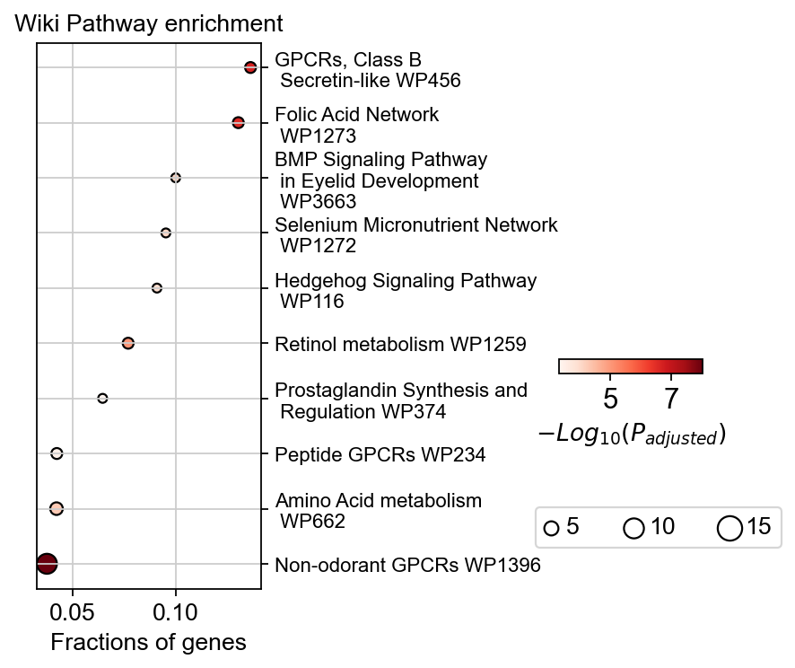
To visualize the enrichment, we use geneset_plot to finish it

ov.bulk.geneset_plot(enr,figsize=(2,5),fig_title='Wiki Pathway enrichment',
                    cax_loc=[2, 0.45, 0.5, 0.02],
                    bbox_to_anchor_used=(-0.25, -13),node_diameter=10,
                     custom_ticks=[5,7],text_knock=3,
                    cmap='Reds')

<AxesSubplot: title={'center': 'Wiki Pathway enrichment'}, xlabel='Fractions of genes'>

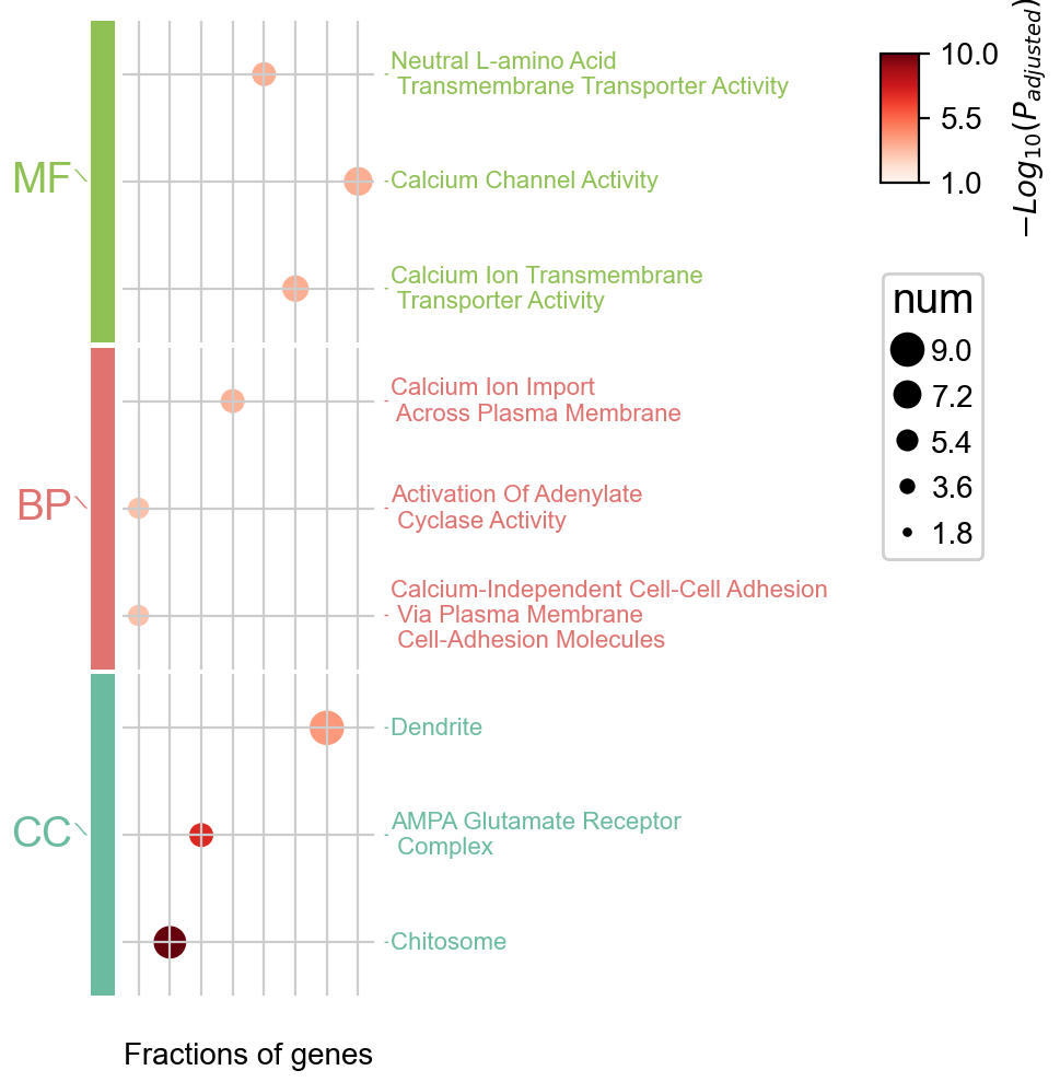
Multi pathway enrichment

In addition to pathway enrichment for a single database, OmicVerse supports enriching and visualizing multiple pathways at the same time, which is implemented using pyComplexHeatmap, and Citetation is welcome!

pathway_dict=ov.utils.geneset_prepare('genesets/GO_Biological_Process_2023.txt',organism='Mouse')
enr_go_bp=ov.bulk.geneset_enrichment(gene_list=deg_genes,
                                pathways_dict=pathway_dict,
                                pvalue_type='auto',
                                organism='mouse')
pathway_dict=ov.utils.geneset_prepare('genesets/GO_Molecular_Function_2023.txt',organism='Mouse')
enr_go_mf=ov.bulk.geneset_enrichment(gene_list=deg_genes,
                                pathways_dict=pathway_dict,
                                pvalue_type='auto',
                                organism='mouse')
pathway_dict=ov.utils.geneset_prepare('genesets/GO_Cellular_Component_2023.txt',organism='Mouse')
enr_go_cc=ov.bulk.geneset_enrichment(gene_list=deg_genes,
                                pathways_dict=pathway_dict,
                                pvalue_type='auto',
                                organism='mouse')

enr_dict={'BP':enr_go_bp,
         'MF':enr_go_mf,
         'CC':enr_go_cc}
colors_dict={
    'BP':ov.pl.red_color[1],
    'MF':ov.pl.green_color[1],
    'CC':ov.pl.blue_color[1],
}
                
ov.bulk.geneset_plot_multi(enr_dict,colors_dict,num=3,
                   figsize=(2,5),
                   text_knock=3,fontsize=8,
                    cmap='Reds'
                  )

Starting plotting..
Starting calculating row orders..
Reordering rows..
Starting calculating col orders..
Reordering cols..
Plotting matrix..
Inferred max_s (max size of scatter point) is: 106.70147475919528
Collecting legends..
Plotting legends..
Estimated legend width: 9.879166666666666 mm

<Axes: ylabel='$−Log_{10}(P_{adjusted})$'>