Batch correction in Bulk RNA-seq or microarray data

Variability in datasets are not only the product of biological processes: they are also the product of technical biases (Lander et al, 1999). ComBat is one of the most widely used tool for correcting those technical biases called batch effects.

pyComBat (Behdenna et al, 2020) is a new Python implementation of ComBat (Johnson et al, 2007), a software widely used for the adjustment of batch effects in microarray data. While the mathematical framework is strictly the same, pyComBat:

• has similar results in terms of batch effects correction;

• is as fast or faster than the R implementation of ComBat and;

• offers new tools for the community to participate in its development.

Paper: pyComBat, a Python tool for batch effects correction in high-throughput molecular data using empirical Bayes methods

Code: https://github.com/epigenelabs/pyComBat

Colab_Reproducibility：https://colab.research.google.com/drive/121bbIiI3j4pTZ3yA_5p8BRkRyGMMmNAq?usp=sharing

import anndata
import pandas as pd
import omicverse as ov
ov.ov_plot_set()

AnnData object with n_obs × n_vars = 17126 × 161

Loading dataset

This minimal usage example illustrates how to use pyComBat in a default setting, and shows some results on ovarian cancer data, freely available on NCBI’s Gene Expression Omnibus, namely:

• GSE18520

• GSE66957

• GSE69428

The corresponding expression files are available on GitHub.

dataset_1 = pd.read_pickle("data/combat/GSE18520.pickle")
adata1=anndata.AnnData(dataset_1.T)
adata1.obs['batch']='1'
adata1

AnnData object with n_obs × n_vars = 63 × 21755
    obs: 'batch'

dataset_2 = pd.read_pickle("data/combat/GSE66957.pickle")
adata2=anndata.AnnData(dataset_2.T)
adata2.obs['batch']='2'
adata2

AnnData object with n_obs × n_vars = 69 × 22115
    obs: 'batch'

dataset_3 = pd.read_pickle("data/combat/GSE69428.pickle")
adata3=anndata.AnnData(dataset_3.T)
adata3.obs['batch']='3'
adata3

AnnData object with n_obs × n_vars = 29 × 21755
    obs: 'batch'

We use the concat function to join the three datasets together and take the intersection for the same genes

adata=anndata.concat([adata1,adata2,adata3],merge='same')
adata

AnnData object with n_obs × n_vars = 161 × 17126
    obs: 'batch'

Removing batch effect

ov.bulk.batch_correction(adata,batch_key='batch')

Found 3 batches.
Adjusting for 0 covariate(s) or covariate level(s).
Standardizing Data across genes.
Fitting L/S model and finding priors.
Finding parametric adjustments.
Adjusting the Data
Storing batch correction result in adata.layers['batch_correction']

Saving results

Raw datasets

raw_data=adata.to_df().T
raw_data.head()

	GSM461348	GSM461349	GSM461350	GSM461351	GSM461352	GSM461353	GSM461354	GSM461355	GSM461356	GSM461357	...	GSM1701044	GSM1701045	GSM1701046	GSM1701047	GSM1701048	GSM1701049	GSM1701050	GSM1701051	GSM1701052	GSM1701053
gene_symbol
A1BG	4.140079	4.589471	4.526200	4.326366	4.141506	4.528423	4.419378	4.345215	4.184150	4.393646	...	3.490229	4.542913	4.654638	4.199212	4.080964	4.114272	3.883770	4.103220	3.883770	3.487520
A1BG-AS1	5.747137	6.130257	5.781449	5.914044	6.277715	5.668244	5.879830	6.013979	5.968187	6.017624	...	4.005230	4.301880	4.509698	4.089223	4.129560	3.867568	4.094032	3.616044	4.307225	3.891060
A1CF	5.026369	5.120523	5.220462	4.828303	5.078094	5.204209	4.865024	5.119230	5.219517	4.706891	...	4.225589	3.530307	3.215182	2.967515	3.012953	3.496765	3.117002	3.072093	2.570765	3.163533
A2M	7.892506	7.730116	7.796338	8.525167	7.545033	7.846979	7.638513	7.487679	7.533089	6.965395	...	10.273206	4.061912	4.393332	4.716536	3.447348	3.134037	4.009413	3.953612	7.664853	3.548574
A2ML1	3.966217	4.482255	3.964664	3.906967	3.952821	3.985276	3.997008	4.101457	4.015285	3.765736	...	2.478731	4.132282	3.952693	2.527621	2.358378	2.414869	2.204600	2.295500	2.167646	2.216867

5 rows × 161 columns

Removing Batch datasets

removing_data=adata.to_df(layer='batch_correction').T
removing_data.head()

	GSM461348	GSM461349	GSM461350	GSM461351	GSM461352	GSM461353	GSM461354	GSM461355	GSM461356	GSM461357	...	GSM1701044	GSM1701045	GSM1701046	GSM1701047	GSM1701048	GSM1701049	GSM1701050	GSM1701051	GSM1701052	GSM1701053
gene_symbol
A1BG	4.223549	4.846659	4.758930	4.481847	4.225527	4.762011	4.610814	4.507982	4.284656	4.575134	...	4.237836	5.378695	5.499778	5.006204	4.878052	4.914150	4.664341	4.902172	4.664341	4.234900
A1BG-AS1	5.730287	6.253722	5.777166	5.958322	6.455185	5.622501	5.911578	6.094858	6.032295	6.099838	...	5.841898	5.990944	6.095359	5.884098	5.904365	5.772731	5.886515	5.646358	5.993630	5.784535
A1CF	3.922941	3.975597	4.031489	3.812171	3.951869	4.022399	3.832708	3.974874	4.030960	3.744271	...	4.229097	3.822095	3.637628	3.492649	3.519248	3.802460	3.580155	3.553867	3.260401	3.607394
A2M	9.488789	9.219466	9.329295	10.538060	8.912504	9.413282	9.067542	8.817383	8.892696	7.951175	...	11.137033	7.182184	7.393206	7.598996	6.790880	6.591389	7.148757	7.113228	9.476245	6.855333
A2ML1	4.317770	5.553678	4.314051	4.175866	4.285686	4.363418	4.391514	4.641670	4.435287	3.837621	...	3.807064	5.766146	5.553374	3.864987	3.664473	3.731402	3.482281	3.589976	3.438499	3.496814

5 rows × 161 columns

save

raw_data.to_csv('raw_data.csv')
removing_data.to_csv('removing_data.csv')

You can also save adata object

adata.write_h5ad('adata_batch.h5ad',compression='gzip')
#adata=ov.read('adata_batch.h5ad')

Compare the dataset before and after correction

We specify three different colours for three different datasets

color_dict={
    '1':ov.utils.red_color[1],
    '2':ov.utils.blue_color[1],
    '3':ov.utils.green_color[1],
}

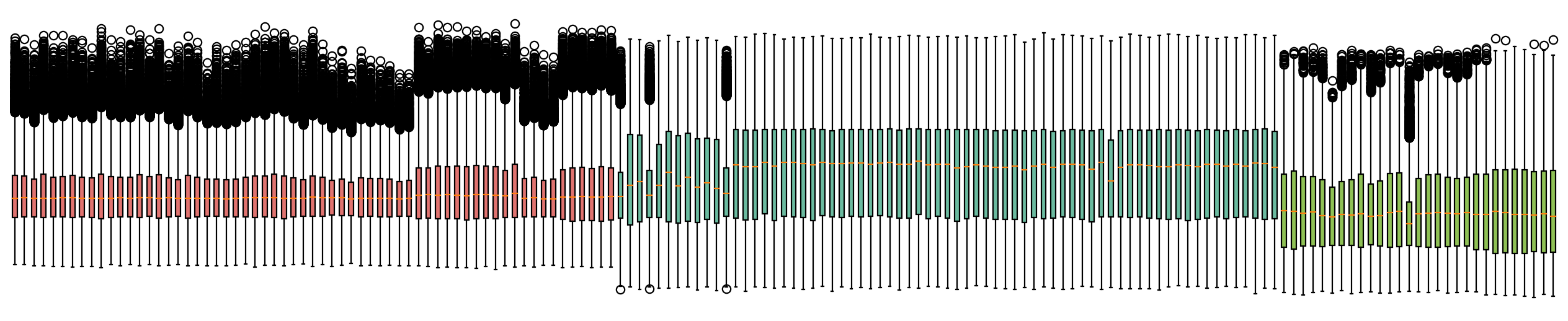
fig,ax=plt.subplots( figsize = (20,4))
bp=plt.boxplot(adata.to_df().T,patch_artist=True)
for i,batch in zip(range(adata.shape[0]),adata.obs['batch']):
    bp['boxes'][i].set_facecolor(color_dict[batch])
ax.axis(False)
plt.show()

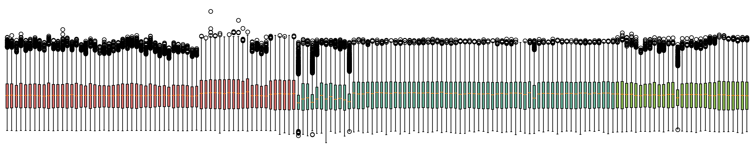
fig,ax=plt.subplots( figsize = (20,4))
bp=plt.boxplot(adata.to_df(layer='batch_correction').T,patch_artist=True)
for i,batch in zip(range(adata.shape[0]),adata.obs['batch']):
    bp['boxes'][i].set_facecolor(color_dict[batch])
ax.axis(False)
plt.show()

In addition to using boxplots to observe the effect of batch removal, we can also use PCA to observe the effect of batch removal

adata.layers['raw']=adata.X.copy()

We first calculate the PCA on the raw dataset

ov.pp.pca(adata,layer='raw',n_pcs=50)
adata

AnnData object with n_obs × n_vars = 161 × 17126
    obs: 'batch'
    uns: 'raw|original|pca_var_ratios', 'raw|original|cum_sum_eigenvalues'
    obsm: 'raw|original|X_pca'
    varm: 'raw|original|pca_loadings'
    layers: 'batch_correction', 'raw', 'lognorm'

We then calculate the PCA on the batch_correction dataset

ov.pp.pca(adata,layer='batch_correction',n_pcs=50)
adata

AnnData object with n_obs × n_vars = 161 × 17126
    obs: 'batch'
    uns: 'raw|original|pca_var_ratios', 'raw|original|cum_sum_eigenvalues', 'batch_correction|original|pca_var_ratios', 'batch_correction|original|cum_sum_eigenvalues'
    obsm: 'raw|original|X_pca', 'batch_correction|original|X_pca'
    varm: 'raw|original|pca_loadings', 'batch_correction|original|pca_loadings'
    layers: 'batch_correction', 'raw', 'lognorm'

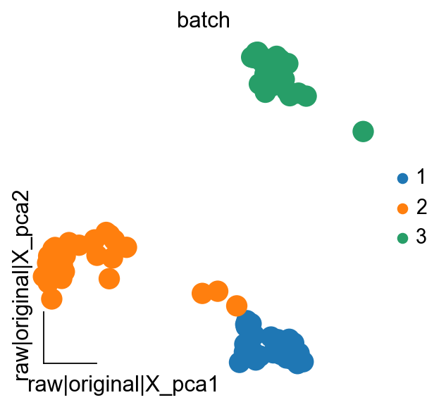
ov.pl.embedding(adata,
                  basis='raw|original|X_pca',
                  color='batch',
                  frameon='small')

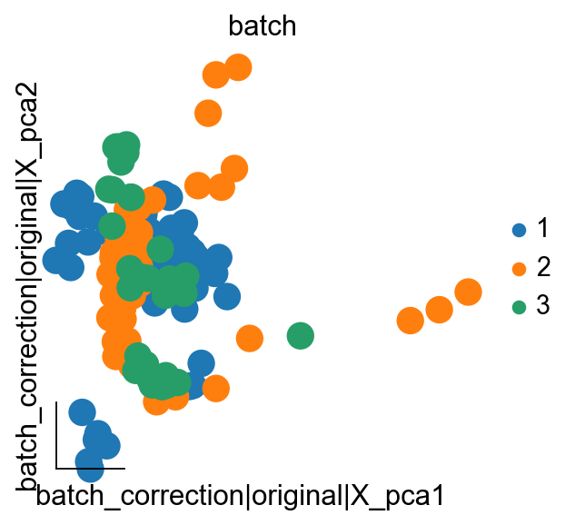
ov.pl.embedding(adata,
                  basis='batch_correction|original|X_pca',
                  color='batch',
                  frameon='small')