Celltype auto annotation with MetaTiME
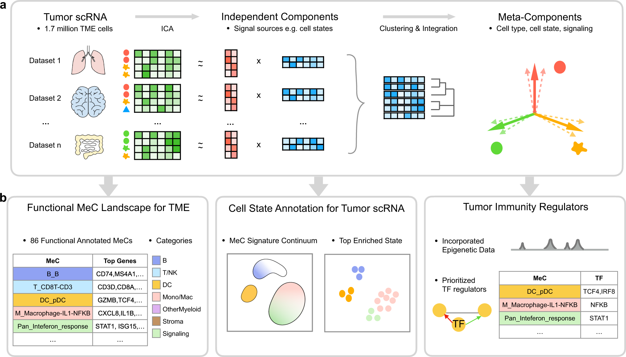
MetaTiME learns data-driven, interpretable, and reproducible gene programs by integrating millions of single cells from hundreds of tumor scRNA-seq data. The idea is to learn a map of single-cell space with biologically meaningful directions from large-scale data, which helps understand functional cell states and transfers knowledge to new data analysis. MetaTiME provides pretrained meta-components (MeCs) to automatically annotate fine-grained cell states and plot signature continuum for new single-cells of tumor microenvironment.
Here, we integrate MetaTiME in omicverse. This tutorial demonstrates how to use MetaTiME (original code) to annotate celltype in TME
Code: https://github.com/yi-zhang/MetaTiME
Colab_Reproducibility:https://colab.research.google.com/drive/1isvjTfSFM2cy6GzHWAwbuvSjveEJijzP?usp=sharing
import omicverse as ov
ov.utils.ov_plot_set()
2023-07-03 20:18:41.594673: I tensorflow/core/platform/cpu_feature_guard.cc:193] This TensorFlow binary is optimized with oneAPI Deep Neural Network Library (oneDNN) to use the following CPU instructions in performance-critical operations:  AVX2 FMA
To enable them in other operations, rebuild TensorFlow with the appropriate compiler flags.
2023-07-03 20:18:42.195329: W tensorflow/compiler/xla/stream_executor/platform/default/dso_loader.cc:64] Could not load dynamic library 'libnvinfer.so.7'; dlerror: libnvinfer.so.7: cannot open shared object file: No such file or directory; LD_LIBRARY_PATH: /usr/local/cudnn/lib:/usr/local/cuda/lib:
2023-07-03 20:18:42.195428: W tensorflow/compiler/xla/stream_executor/platform/default/dso_loader.cc:64] Could not load dynamic library 'libnvinfer_plugin.so.7'; dlerror: libnvinfer_plugin.so.7: cannot open shared object file: No such file or directory; LD_LIBRARY_PATH: /usr/local/cudnn/lib:/usr/local/cuda/lib:
2023-07-03 20:18:42.195434: W tensorflow/compiler/tf2tensorrt/utils/py_utils.cc:38] TF-TRT Warning: Cannot dlopen some TensorRT libraries. If you would like to use Nvidia GPU with TensorRT, please make sure the missing libraries mentioned above are installed properly.
/mnt/data/env/pyomic/lib/python3.8/site-packages/phate/__init__.py
Data normalize and Batch remove
The sample data has multiple patients , and we can use batch correction on patients. Here, we using scVI to remove batch.
Note
If your data contains count matrix, we provide a wrapped function for pre-processing the data. Otherwise, if the data is already depth-normalized, log-transformed, and cells are filtered, we can skip this step.
'''
import scvi
scvi.model.SCVI.setup_anndata(adata, layer="counts", batch_key="patient")
vae = scvi.model.SCVI(adata, n_layers=2, n_latent=30, gene_likelihood="nb")
vae.train()
adata.obsm["X_scVI"] = vae.get_latent_representation()
'''
Example data can be obtained from figshare: https://figshare.com/ndownloader/files/41440050
import scanpy as sc
adata=sc.read('TiME_adata_scvi.h5ad')
adata
AnnData object with n_obs × n_vars = 40911 × 2000
    obs: 'RNA_snn_res_1', 'assign_ident', 'assign_score', 'nCount_RNA', 'nFeature_RNA', 'orig_ident', 'patient', 'seurat_clusters', 'treatment', 'n_counts', 'log_counts', 'n_genes', 'n_genes_by_counts', 'total_counts', 'total_counts_mt', 'pct_counts_mt', 'isTME'
    var: 'Selected', 'vst_mean', 'vst_variable', 'vst_variance', 'vst_variance_expected', 'vst_variance_standardized', 'n_cells', 'mt', 'n_cells_by_counts', 'mean_counts', 'pct_dropout_by_counts', 'total_counts', 'highly_variable', 'means', 'dispersions', 'dispersions_norm', 'highly_variable_rank', 'variances', 'variances_norm', 'highly_variable_nbatches'
    uns: 'hvg'
    obsm: 'X_scVI'
    varm: 'PCs'
    layers: 'counts'
It is recommended that malignant cells are identified first and removed for best practice in cell state annotation.
In the BCC data, the cluster of malignant cells are identified with inferCNV. We can use the pre-saved column 'isTME' to keep Tumor Microenvironment cells.
These are the authors' exact words, but tests have found that the difference in annotation effect is not that great even without removing the malignant cells
But I think this step is not necessary
#adata = adata[adata.obs['isTME']]
Neighborhood graph calculated
We note that scVI was used earlier to remove the batch effect from the data, so we need to recalculate the neighbourhood map based on what is stored in adata.obsm['X_scVI']. Note that if you are not using scVI but using another method to calculate the neighbourhood map, such as X_pca, then you need to change X_scVI to X_pca to complete the calculation
#Example
#sc.tl.pca(adata)
#sc.pp.neighbors(adata, use_rep="X_pca")
sc.pp.neighbors(adata, use_rep="X_scVI")
computing neighbors
    finished: added to `.uns['neighbors']`
    `.obsp['distances']`, distances for each pair of neighbors
    `.obsp['connectivities']`, weighted adjacency matrix (0:00:18)
To visualize the PCA’s embeddings, we use the pymde package wrapper in omicverse. This is an alternative to UMAP that is GPU-accelerated.
adata.obsm["X_mde"] = ov.utils.mde(adata.obsm["X_scVI"])
#adata.write_h5ad('adata_mde.h5ad',compression='gzip')
#adata=sc.read('adata_mde.h5ad')
MeteTiME model init
Next, let's load the pre-computed MetaTiME MetaComponents (MeCs), and their functional annotation.
TiME_object=ov.single.MetaTiME(adata,mode='table')
...load pre-trained MeCs
...load functional annotation for MetaTiME-TME
We can over-cluster the cells which is useful for fine-grained cell state annotation.
As the resolution gets larger, the number of clusters gets larger
TiME_object.overcluster(resolution=8,clustercol = 'overcluster',)
...overclustering using leiden
running Leiden clustering
    finished: found 111 clusters and added
    'overcluster', the cluster labels (adata.obs, categorical) (0:00:11)
TME celltype predicted
We using TiME_object.predictTiME() to predicted the latent celltype in TME.
- The minor celltype will be stored in
adata.obs['MetaTiME'] - The major celltype will be stored in
adata.obs['Major_MetaTiME']
TiME_object.predictTiME(save_obs_name='MetaTiME')
...projecting MeC scores
......The predicted celltype have been saved in obs.MetaTiME
......The predicted major celltype have been saved in obs.Major_MetaTiME
AnnData object with n_obs × n_vars = 38836 × 2000
    obs: 'RNA_snn_res_1', 'assign_ident', 'assign_score', 'nCount_RNA', 'nFeature_RNA', 'orig_ident', 'patient', 'seurat_clusters', 'treatment', 'n_counts', 'log_counts', 'n_genes', 'n_genes_by_counts', 'total_counts', 'total_counts_mt', 'pct_counts_mt', 'isTME', 'MeC_0', 'MeC_1', 'MeC_2', 'MeC_3', 'MeC_4', 'MeC_5', 'MeC_6', 'MeC_7', 'MeC_8', 'MeC_9', 'MeC_11', 'MeC_12', 'MeC_13', 'MeC_14', 'MeC_15', 'MeC_16', 'MeC_17', 'MeC_18', 'MeC_19', 'MeC_20', 'MeC_21', 'MeC_22', 'MeC_23', 'MeC_24', 'MeC_25', 'MeC_26', 'MeC_27', 'MeC_28', 'MeC_29', 'MeC_30', 'MeC_31', 'MeC_32', 'MeC_33', 'MeC_34', 'MeC_35', 'MeC_36', 'MeC_37', 'MeC_38', 'MeC_39', 'MeC_40', 'MeC_41', 'MeC_42', 'MeC_43', 'MeC_45', 'MeC_46', 'MeC_47', 'MeC_48', 'MeC_49', 'MeC_50', 'MeC_51', 'MeC_52', 'MeC_53', 'MeC_54', 'MeC_55', 'MeC_56', 'MeC_57', 'MeC_58', 'MeC_59', 'MeC_61', 'MeC_63', 'MeC_64', 'MeC_65', 'MeC_66', 'MeC_67', 'MeC_68', 'MeC_69', 'MeC_74', 'MeC_75', 'MeC_76', 'MeC_77', 'MeC_78', 'MeC_81', 'MeC_83', 'overcluster', 'MetaTiME_overcluster', 'MetaTiME', 'Major_MetaTiME'
    var: 'Selected', 'vst_mean', 'vst_variable', 'vst_variance', 'vst_variance_expected', 'vst_variance_standardized', 'n_cells', 'mt', 'n_cells_by_counts', 'mean_counts', 'pct_dropout_by_counts', 'total_counts', 'highly_variable', 'means', 'dispersions', 'dispersions_norm', 'highly_variable_rank', 'variances', 'variances_norm', 'highly_variable_nbatches'
    uns: 'hvg', 'neighbors', 'patient_colors', 'leiden'
    obsm: 'X_mde', 'X_scVI'
    varm: 'PCs'
    layers: 'counts'
    obsp: 'connectivities', 'distances'
Visualize
The original author provides a drawing function that effectively avoids overlapping labels. Here I have expanded its parameters so that it can be visualised using parameters other than X_umap
We can also use sc.pl.embedding to visualize the celltype
