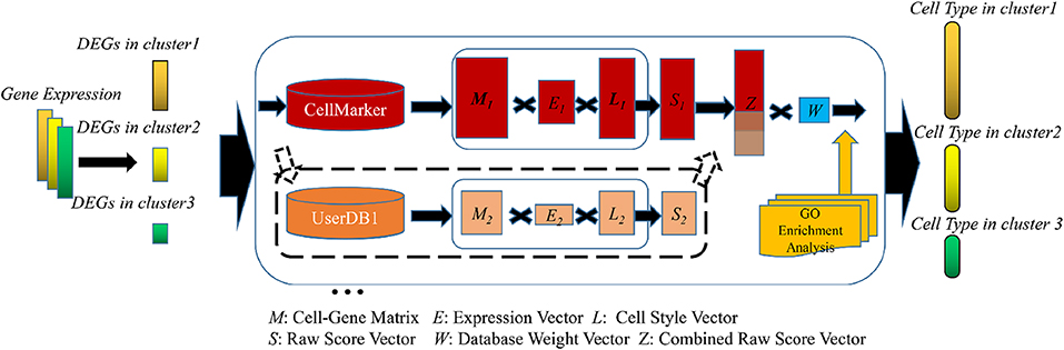
Celltype auto annotation with SCSA
Single-cell transcriptomics allows the analysis of thousands of cells in a single experiment and the identification of novel cell types, states and dynamics in a variety of tissues and organisms. Standard experimental protocols and analytical workflows have been developed to create single-cell transcriptomic maps from tissues.
This tutorial focuses on how to interpret this data to identify cell types, states, and other biologically relevant patterns with the goal of creating annotated cell maps.
Paper: SCSA: A Cell Type Annotation Tool for Single-Cell RNA-seq Data
Code: https://github.com/bioinfo-ibms-pumc/SCSA
Colab_Reproducibility:https://colab.research.google.com/drive/1BC6hPS0CyBhNu0BYk8evu57-ua1bAS0T?usp=sharing
Note
The annotation with SCSA can’t be used in rare celltype annotations
import scanpy as sc
print(f'scanpy version:{sc.__version__}')
import omicverse as ov
print(f'omicverse version:{ov.__version__}')
ov.ov_plot_set()
scanpy version:1.10.3

   ____            _     _    __
  / __ \____ ___  (_)___| |  / /__  _____________
 / / / / __ `__ \/ / ___/ | / / _ \/ ___/ ___/ _ \
/ /_/ / / / / / / / /__ | |/ /  __/ /  (__  )  __/
\____/_/ /_/ /_/_/\___/ |___/\___/_/  /____/\___/

Version: 1.6.9, Tutorials: https://omicverse.readthedocs.io/
omicverse version:1.6.9
Dependency error: (pydeseq2 0.4.11 (/mnt/home/zehuazeng/software/rsc/lib/python3.10/site-packages), Requirement.parse('pydeseq2<=0.4.0,>=0.3'))
Loading data
The data consist of 3k PBMCs from a Healthy Donor and are freely available from 10x Genomics (here from this webpage). On a unix system, you can uncomment and run the following to download and unpack the data. The last line creates a directory for writing processed data.
# !mkdir data
# !wget http://cf.10xgenomics.com/samples/cell-exp/1.1.0/pbmc3k/pbmc3k_filtered_gene_bc_matrices.tar.gz -O data/pbmc3k_filtered_gene_bc_matrices.tar.gz
# !cd data; tar -xzf pbmc3k_filtered_gene_bc_matrices.tar.gz
# !mkdir write
Read in the count matrix into an AnnData object, which holds many slots for annotations and different representations of the data. It also comes with its own HDF5-based file format: .h5ad.
adata = sc.read_10x_mtx(
    'data/filtered_gene_bc_matrices/hg19/',  # the directory with the `.mtx` file
    var_names='gene_symbols',                # use gene symbols for the variable names (variables-axis index)
    cache=True)                              # write a cache file for faster subsequent reading
... reading from cache file cache/data-filtered_gene_bc_matrices-hg19-matrix.h5ad
Data preprocessing
Here, we use ov.single.scanpy_lazy to preprocess the raw data of scRNA-seq, it included filter the doublets cells, normalizing counts per cell, log1p, extracting highly variable genes, and cluster of cells calculation.
But if you want to experience step-by-step preprocessing, we also provide more detailed preprocessing steps here, please refer to our preprocess chapter for a detailed explanation.
We stored the raw counts in count layers, and the raw data in adata.raw.to_adata().
#adata=ov.single.scanpy_lazy(adata)

#quantity control
adata=ov.pp.qc(adata,
              tresh={'mito_perc': 0.05, 'nUMIs': 500, 'detected_genes': 250})
#normalize and high variable genes (HVGs) calculated
adata=ov.pp.preprocess(adata,mode='shiftlog|pearson',n_HVGs=2000,)

#save the whole genes and filter the non-HVGs
adata.raw = adata
adata = adata[:, adata.var.highly_variable_features]

#scale the adata.X
ov.pp.scale(adata)

#Dimensionality Reduction
ov.pp.pca(adata,layer='scaled',n_pcs=50)

#Neighbourhood graph construction
sc.pp.neighbors(adata, n_neighbors=15, n_pcs=50,
               use_rep='scaled|original|X_pca')

#clusters
sc.tl.leiden(adata)

#Dimensionality Reduction for visualization(X_mde=X_umap+GPU)
adata.obsm["X_mde"] = ov.utils.mde(adata.obsm["scaled|original|X_pca"])
adata
CPU mode activated
Calculate QC metrics
End calculation of QC metrics.
Original cell number: 2700
!!!It should be noted that the `scrublet` detection is too old and             may not work properly.!!!
!!!if you want to use novel doublet detection,             please set `doublets_method=sccomposite`!!!
Begin of post doublets removal and QC plot using`scrublet`
Running Scrublet
filtered out 19024 genes that are detected in less than 3 cells
normalizing counts per cell
    finished (0:00:00)
extracting highly variable genes
    finished (0:00:00)
--> added
    'highly_variable', boolean vector (adata.var)
    'means', float vector (adata.var)
    'dispersions', float vector (adata.var)
    'dispersions_norm', float vector (adata.var)
normalizing counts per cell
    finished (0:00:00)
normalizing counts per cell
    finished (0:00:00)
Embedding transcriptomes using PCA...
    using data matrix X directly
Automatically set threshold at doublet score = 0.23
Detected doublet rate = 1.5%
Estimated detectable doublet fraction = 37.4%
Overall doublet rate:
	Expected   = 5.0%
	Estimated  = 4.1%
    Scrublet finished (0:00:02)
Cells retained after scrublet: 2659, 41 removed.
End of post doublets removal and QC plots.
Filters application (seurat or mads)
Lower treshold, nUMIs: 500; filtered-out-cells:         0
Lower treshold, n genes: 250; filtered-out-cells:         3
Lower treshold, mito %: 0.05; filtered-out-cells:         56
Filters applicated.
Total cell filtered out with this last --mode seurat QC (and its     chosen options): 59
Cells retained after scrublet and seurat filtering: 2600, 100 removed.
filtered out 19112 genes that are detected in less than 3 cells
Begin robust gene identification
After filtration, 13626/13626 genes are kept.     Among 13626 genes, 13626 genes are robust.
End of robust gene identification.
Begin size normalization: shiftlog and HVGs selection pearson
normalizing counts per cell. The following highly-expressed genes are not considered during normalization factor computation:
[]
    finished (0:00:00)
extracting highly variable genes
--> added
    'highly_variable', boolean vector (adata.var)
    'highly_variable_rank', float vector (adata.var)
    'highly_variable_nbatches', int vector (adata.var)
    'highly_variable_intersection', boolean vector (adata.var)
    'means', float vector (adata.var)
    'variances', float vector (adata.var)
    'residual_variances', float vector (adata.var)
Time to analyze data in cpu: 1.1343843936920166 seconds.
End of size normalization: shiftlog and HVGs selection pearson
... as `zero_center=True`, sparse input is densified and may lead to large memory consumption
computing PCA
    with n_comps=50
    finished (0:00:00)
computing neighbors
    finished: added to `.uns['neighbors']`
    `.obsp['distances']`, distances for each pair of neighbors
    `.obsp['connectivities']`, weighted adjacency matrix (0:00:05)
running Leiden clustering
    finished: found 11 clusters and added
    'leiden', the cluster labels (adata.obs, categorical) (0:00:00)
AnnData object with n_obs × n_vars = 2600 × 2000
    obs: 'nUMIs', 'mito_perc', 'detected_genes', 'cell_complexity', 'doublet_score', 'predicted_doublet', 'passing_mt', 'passing_nUMIs', 'passing_ngenes', 'n_genes', 'leiden'
    var: 'gene_ids', 'mt', 'n_cells', 'percent_cells', 'robust', 'means', 'variances', 'residual_variances', 'highly_variable_rank', 'highly_variable_features'
    uns: 'scrublet', 'log1p', 'hvg', 'pca', 'scaled|original|pca_var_ratios', 'scaled|original|cum_sum_eigenvalues', 'neighbors', 'leiden'
    obsm: 'X_pca', 'scaled|original|X_pca', 'X_mde'
    varm: 'PCs', 'scaled|original|pca_loadings'
    layers: 'counts', 'scaled'
    obsp: 'distances', 'connectivities'
Cell annotate automatically
We create a pySCSA object from the adata, and we need to set some parameter to annotate correctly.
In normal annotate, we set celltype='normal' and target='cellmarker' or 'panglaodb' to perform the cell annotate.
But in cancer annotate, we need to set the celltype='cancer' and target='cancersea' to perform the cell annotate.
Note
The annotation with SCSA need to download the database at first. It can be downloaded automatically. But sometimes you will have problems with network errors.
2023 Version (build on pandas<=1.5.3): The database can be downloaded from figshare, Google Drive and 百度云.
2024 Version (build on pandas>2): The database can be downloaded from Google Drive and 百度云.
And you need to set parameter model_path='path'
The database create code could be found in scsa_database_create.ipynb. Thanks for @fredsamhaak @H1207953831 in issue #232 #176
scsa=ov.single.pySCSA(adata=adata,
                      foldchange=1.5,
                      pvalue=0.01,
                      celltype='normal',
                      target='cellmarker',
                      tissue='All',
                      model_path='temp/pySCSA_2024_v1_plus.db'
)
In the previous cell clustering we used the leiden algorithm, so here we specify that the type is set to leiden. if you are using louvain, please change it. And, we will annotate all clusters, if you only want to annotate a few of the classes, please follow '[1]', '[1,2,3]', '[...]' Enter in the format.
rank_rep means the sc.tl.rank_genes_groups(adata, clustertype, method='wilcoxon'), if we provided the rank_genes_groups in adata.uns, rank_rep can be set as False
anno=scsa.cell_anno(clustertype='leiden',
               cluster='all',rank_rep=True)
ranking genes
    finished (0:00:01)
...Auto annotate cell
Version V2.2 [2024/12/18]
DB load: GO_items:47347,Human_GO:3,Mouse_GO:3,
CellMarkers:82887,CancerSEA:1574,
Ensembl_HGNC:61541,Ensembl_Mouse:55414
<omicverse.single._SCSA.Annotator object at 0x7f879295aad0>
Version V2.2 [2024/12/18]
DB load: GO_items:47347,Human_GO:3,Mouse_GO:3,
CellMarkers:82887,CancerSEA:1574,
Ensembl_HGNC:61541,Ensembl_Mouse:55414
load markers: 70276
Cluster 0 Gene number: 149
Other Gene number: 1524
Cluster 1 Gene number: 65
Other Gene number: 1579
Cluster 10 Gene number: 123
Other Gene number: 1557
Cluster 2 Gene number: 518
Other Gene number: 1513
Cluster 3 Gene number: 129
Other Gene number: 1532
Cluster 4 Gene number: 83
Other Gene number: 1586
Cluster 5 Gene number: 920
Other Gene number: 1284
Cluster 6 Gene number: 244
Other Gene number: 1498
Cluster 7 Gene number: 4
Other Gene number: 1601
Cluster 8 Gene number: 62
Other Gene number: 1601
Cluster 9 Gene number: 569
Other Gene number: 1390
#Cluster Type Celltype Score Times
['0', '?', 'T cell|CD4+ T cell', '13.178917022960926|6.8061709979163005', 1.9363188240488862]
['1', '?', 'T cell|Naive CD8+ T cell', '8.44505754473862|5.156218870163674', 1.6378392301393032]
['10', 'Good', 'Megakaryocyte', 10.334648914788692, 2.029183977014163]
['2', '?', 'Monocyte|Macrophage', '14.764576625686557|8.789587478708638', 1.6797803834880043]
['3', 'Good', 'B cell', 13.812808366659368, 3.97118749472909]
['4', '?', 'Natural killer cell|T cell', '8.698876988328609|7.9591723394151535', 1.092937383105818]
['5', '?', 'Monocyte|Macrophage', '13.989335587848112|9.940008439379591', 1.4073766308312372]
['6', 'Good', 'Natural killer cell', 15.589448201913797, 3.6505468200421314]
['7', '?', 'T cell|Natural killer cell', '5.007589020260128|3.635144325168466', 1.37754888728608]
['8', 'Good', 'Monocyte', 10.986485157084731, 2.2059005457967578]
['9', '?', 'Dendritic cell|Monocyte', '8.486516254407464|7.5372353894337465', 1.1259454980408983]
We can query only the better annotated results
scsa.cell_auto_anno(adata,key='scsa_celltype_cellmarker')
...cell type added to scsa_celltype_cellmarker on obs of anndata
We can also use panglaodb as target to annotate the celltype
scsa=ov.single.pySCSA(adata=adata,
                          foldchange=1.5,
                          pvalue=0.01,
                          celltype='normal',
                          target='panglaodb',
                          tissue='All',
                          model_path='temp/pySCSA_2024_v1_plus.db'

)
res=scsa.cell_anno(clustertype='leiden',
               cluster='all',rank_rep=True)
ranking genes
    finished (0:00:01)
...Auto annotate cell
Version V2.2 [2024/12/18]
DB load: GO_items:47347,Human_GO:3,Mouse_GO:3,
CellMarkers:82887,CancerSEA:1574,PanglaoDB:24223
Ensembl_HGNC:61541,Ensembl_Mouse:55414
<omicverse.single._SCSA.Annotator object at 0x7f87933d9570>
Version V2.2 [2024/12/18]
DB load: GO_items:47347,Human_GO:3,Mouse_GO:3,
CellMarkers:82887,CancerSEA:1574,PanglaoDB:24223
Ensembl_HGNC:61541,Ensembl_Mouse:55414
load markers: 70276
Cluster 0 Gene number: 149
Other Gene number: 669
Cluster 1 Gene number: 65
Other Gene number: 698
Cluster 10 Gene number: 123
Other Gene number: 672
Cluster 2 Gene number: 518
Other Gene number: 660
Cluster 3 Gene number: 129
Other Gene number: 661
Cluster 4 Gene number: 83
Other Gene number: 699
Cluster 5 Gene number: 920
Other Gene number: 611
Cluster 6 Gene number: 244
Other Gene number: 656
Cluster 7 Gene number: 4
Other Gene number: 709
Cluster 8 Gene number: 62
Other Gene number: 709
Cluster 9 Gene number: 569
Other Gene number: 671
#Cluster Type Celltype Score Times
['0', '?', 'T Cells|T Memory Cells', '3.5600750455818564|3.1097642366140383', 1.1448054497720135]
['1', '?', 'T Cells|T Memory Cells', '3.40627617083116|3.205891183442281', 1.0625052367416035]
['10', 'Good', 'Platelets', 7.433149861365802, 2.436479042204059]
['2', '?', 'Monocytes|Alveolar Macrophages', '3.7036208808369846|2.930737286401599', 1.2637164368234257]
['3', '?', 'B Cells Naive|B Cells Memory', '4.329420431801275|3.955259450025973', 1.0945983408933755]
['4', '?', 'NK Cells|T Cells', '3.008115828143599|2.7009557062706313', 1.1137227541939523]
['5', '?', 'Monocytes|Macrophages', '3.7593052491537016|2.8292867080893154', 1.3287113103120078]
['6', '?', 'NK Cells|Decidual Cells', '4.1134016043498995|2.8564096383637296', 1.4400601192153333]
['7', '?', 'Decidual Cells|NK Cells', '1.601349011754446|1.601349011754446', 1.0]
['8', '?', 'Monocytes|Alveolar Macrophages', '2.675429836435337|2.09584715260779', 1.276538622154002]
['9', '?', 'Dendritic Cells|Langerhans Cells', '3.931944721464753|3.668461896450284', 1.0718237867672615]
We can query only the better annotated results
scsa.cell_anno_print()
Cluster:0	Cell_type:T Cells|T Memory Cells	Z-score:3.56|3.11
Cluster:1	Cell_type:T Cells|T Memory Cells	Z-score:3.406|3.206
Cluster:2	Cell_type:Monocytes|Alveolar Macrophages	Z-score:3.704|2.931
Cluster:3	Cell_type:B Cells Naive|B Cells Memory	Z-score:4.329|3.955
Cluster:4	Cell_type:NK Cells|T Cells	Z-score:3.008|2.701
Cluster:5	Cell_type:Monocytes|Macrophages	Z-score:3.759|2.829
Cluster:6	Cell_type:NK Cells|Decidual Cells	Z-score:4.113|2.856
Cluster:7	Cell_type:Decidual Cells|NK Cells	Z-score:1.601|1.601
Cluster:8	Cell_type:Monocytes|Alveolar Macrophages	Z-score:2.675|2.096
Cluster:9	Cell_type:Dendritic Cells|Langerhans Cells	Z-score:3.932|3.668
Nice:Cluster:10	Cell_type:Platelets	Z-score:7.433
scsa.cell_auto_anno(adata,key='scsa_celltype_panglaodb')
...cell type added to scsa_celltype_panglaodb on obs of anndata
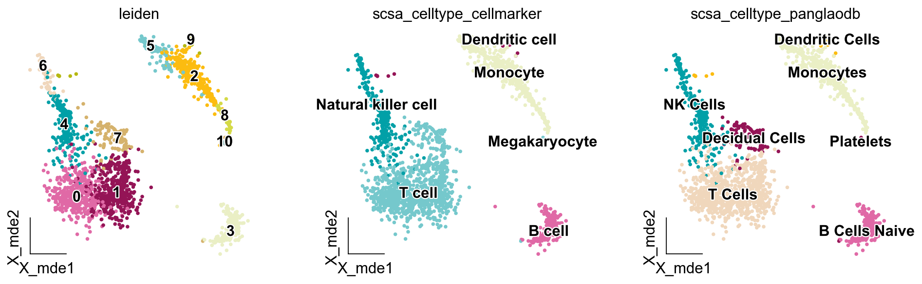
Here, we introduce the dimensionality reduction visualisation function ov.utils.embedding, which is similar to scanpy.pl.embedding, except that when we set frameon='small', we scale the axes to the bottom-left corner and scale the colourbar to the bottom-right corner.
adata: the anndata object
basis: the visualized embedding stored in adata.obsm
color: the visualized obs/var
legend_loc: the location of legend, if you set None, it will be visualized in right.
frameon: it can be set
small, False or Nonelegend_fontoutline: the outline in the text of legend.
palette: Different categories of colours, we have a number of different colours preset in omicverse, including
ov.utils.palette(),ov.utils.red_color,ov.utils.blue_color,ov.utils.green_color,ov. utils.orange_color. The preset colours can help you achieve a more beautiful visualisation.
ov.utils.embedding(adata,
                   basis='X_mde',
                   color=['leiden','scsa_celltype_cellmarker','scsa_celltype_panglaodb'],
                   legend_loc='on data',
                   frameon='small',
                   legend_fontoutline=2,
                   palette=ov.utils.palette()[14:],
                  )
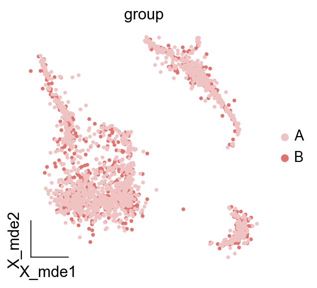
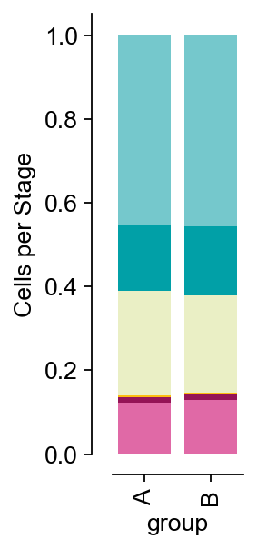
If you want to draw stacked histograms of cell type proportions, you first need to colour the groups you intend to draw using ov.utils.embedding. Then use ov.utils.plot_cellproportion to specify the groups you want to plot, and you can see a plot of cell proportions in the different groups
#Randomly designate the first 1000 cells as group B and the rest as group A
adata.obs['group']='A'
adata.obs.loc[adata.obs.index[:1000],'group']='B'
#Colored
ov.utils.embedding(adata,
                   basis='X_mde',
                   color=['group'],
                   frameon='small',legend_fontoutline=2,
                   palette=ov.utils.red_color,
                  )
ov.utils.plot_cellproportion(adata=adata,celltype_clusters='scsa_celltype_cellmarker',
                    visual_clusters='group',
                    visual_name='group',figsize=(2,4))
(<Figure size 160x320 with 1 Axes>,
 <AxesSubplot: xlabel='group', ylabel='Cells per Stage'>)
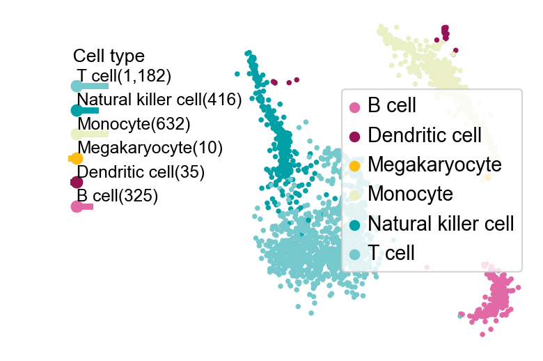
Of course, we also provide another downscaled visualisation of the graph using ov.utils.plot_embedding_celltype
ov.utils.plot_embedding_celltype(adata,figsize=None,basis='X_mde',
                            celltype_key='scsa_celltype_cellmarker',
                            title='            Cell type',
                            celltype_range=(2,6),
                            embedding_range=(4,10))
(<Figure size 480x320 with 2 Axes>,
 [<AxesSubplot: xlabel='X_mde1', ylabel='X_mde2'>, <AxesSubplot: >])
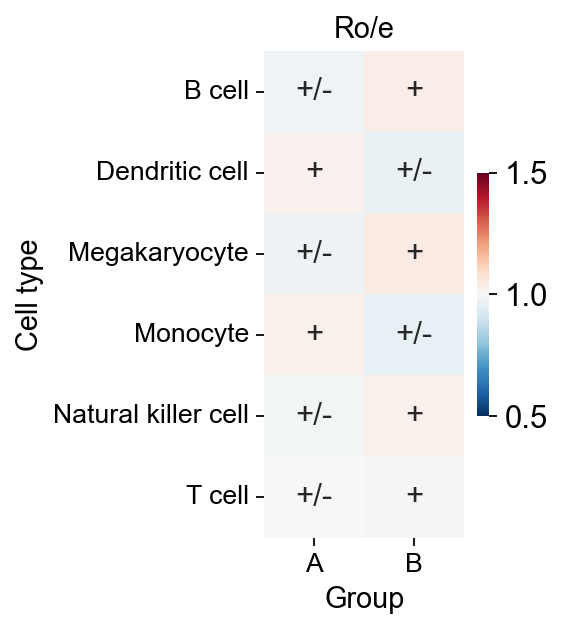
We calculated the ratio of observed to expected cell numbers (Ro/e) for each cluster in different tissues to quantify the tissue preference of each cluster (Guo et al., 2018; Zhang et al., 2018). The expected cell num- bers for each combination of cell clusters and tissues were obtained from the chi-square test. One cluster was identified as being enriched in a specific tissue if Ro/e>1.
The Ro/e function was wrote by Haihao Zhang.
roe=ov.utils.roe(adata,sample_key='group',cell_type_key='scsa_celltype_cellmarker')
chi2: 1.1053770301508763, dof: 5, pvalue: 0.953626625332813
P-value is greater than 0.05, there is no statistical significance
import seaborn as sns
import matplotlib.pyplot as plt
fig, ax = plt.subplots(figsize=(2,4))

transformed_roe = roe.copy()
transformed_roe = transformed_roe.applymap(
    lambda x: '+++' if x >= 2 else ('++' if x >= 1.5 else ('+' if x >= 1 else '+/-')))

sns.heatmap(roe, annot=transformed_roe, cmap='RdBu_r', fmt='',
            cbar=True, ax=ax,vmin=0.5,vmax=1.5,cbar_kws={'shrink':0.5})
plt.xticks(fontsize=12)
plt.yticks(fontsize=12)

plt.xlabel('Group',fontsize=13)
plt.ylabel('Cell type',fontsize=13)
plt.title('Ro/e',fontsize=13)
Text(0.5, 1.0, 'Ro/e')
Cell annotate manually
In order to compare the accuracy of our automatic annotations, we will here use marker genes to manually annotate the cluster and compare the accuracy of the pySCSA and manual.
We need to prepare a marker’s dict at first
res_marker_dict={
    'Megakaryocyte':['ITGA2B','ITGB3'],
    'Dendritic cell':['CLEC10A','IDO1'],
    'Monocyte' :['S100A8','S100A9','LST1',],
    'Macrophage':['CSF1R','CD68'],
    'B cell':['MS4A1','CD79A','MZB1',],
    'NK/NKT cell':['GNLY','KLRD1'],
    'CD8+T cell':['CD8A','CD8B'],
    'Treg':['CD4','CD40LG','IL7R','FOXP3','IL2RA'],
    'CD4+T cell':['PTPRC','CD3D','CD3E'],

}
We then calculated the expression of marker genes in each cluster and the fraction
sc.tl.dendrogram(adata,'leiden')
sc.pl.dotplot(adata, res_marker_dict, 'leiden',
              dendrogram=True,standard_scale='var')
    using 'X_pca' with n_pcs = 50
Storing dendrogram info using `.uns['dendrogram_leiden']`
WARNING: Groups are not reordered because the `groupby` categories and the `var_group_labels` are different.
categories: 0, 1, 2, etc.
var_group_labels: Megakaryocyte, Dendritic cell, Monocyte, etc.
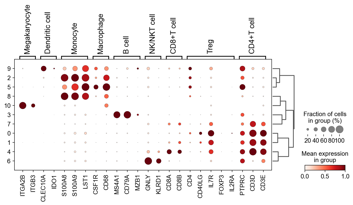
Based on the dotplot, we name each cluster according ov.single.scanpy_cellanno_from_dict
# create a dictionary to map cluster to annotation label
cluster2annotation = {
     '0': 'T cell',
     '1': 'T cell',
     '2': 'Monocyte',#Germ-cell(Oid)
     '3': 'B cell',#Germ-cell(Oid)
     '4': 'T cell',
     '5': 'Macrophage',
     '6': 'NKT cells',
     '7': 'T cell',
    '8':'Monocyte',
    '9':'Dendritic cell',
    '10':'Megakaryocyte',

}
ov.single.scanpy_cellanno_from_dict(adata,anno_dict=cluster2annotation,
                                       clustertype='leiden')
...cell type added to major_celltype on obs of anndata
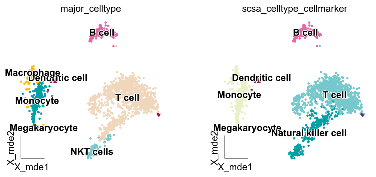
Compare the pySCSA and Manual
We can see that the auto-annotation results are almost identical to the manual annotation, the only difference is between monocyte and macrophages, but in the previous auto-annotation results, pySCSA gives the option of monocyte|macrophage, so it can be assumed that pySCSA performs better on the pbmc3k data
ov.utils.embedding(adata,
                   basis='X_mde',
                   color=['major_celltype','scsa_celltype_cellmarker'],
                   legend_loc='on data', frameon='small',legend_fontoutline=2,
                   palette=ov.utils.palette()[14:],
                  )
We can use get_celltype_marker to obtain the marker of each celltype
marker_dict=ov.single.get_celltype_marker(adata,clustertype='scsa_celltype_cellmarker')
marker_dict.keys()
...get cell type marker
ranking genes
    finished (0:00:01)
dict_keys(['B cell', 'Dendritic cell', 'Megakaryocyte', 'Monocyte', 'Natural killer cell', 'T cell'])
marker_dict['B cell']
array(['CD74', 'CD79A', 'HLA-DRA', 'CD79B', 'HLA-DPB1', 'HLA-DQA1',
       'MS4A1', 'HLA-DQB1', 'HLA-DRB1', 'CD37', 'HLA-DPA1', 'HLA-DRB5',
       'TCL1A'], dtype=object)
The tissue name in database
For annotation of cell types in specific tissues, we can query the tissues available in the database using get_model_tissue.
scsa.get_model_tissue()
Version V2.1 [2023/06/27]
DB load: GO_items:47347,Human_GO:3,Mouse_GO:3,
CellMarkers:82887,CancerSEA:1574,PanglaoDB:24223
Ensembl_HGNC:61541,Ensembl_Mouse:55414
########################################################################################################################
------------------------------------------------------------------------------------------------------------------------
Species:Human      Num:298
------------------------------------------------------------------------------------------------------------------------
  1: Abdomen                              2: Abdominal adipose tissue             3: Abdominal fat pad
  4: Acinus                               5: Adipose tissue                       6: Adrenal gland
  7: Adventitia                           8: Airway                               9: Airway epithelium
 10: Allocortex                          11: Alveolus                            12: Amniotic fluid
 13: Amniotic membrane                   14: Ampullary                           15: Anogenital tract
 16: Antecubital vein                    17: Anterior cruciate ligament          18: Anterior presomitic mesoderm
 19: Aorta                               20: Aortic valve                        21: Artery
 22: Arthrosis                           23: Articular Cartilage                 24: Ascites
 25: Ascitic fluid                       26: Atrium                              27: Basal airway
 28: Basilar membrane                    29: Beige Fat                           30: Bile duct
 31: Biliary tract                       32: Bladder                             33: Blood
 34: Blood vessel                        35: Bone                                36: Bone marrow
 37: Brain                               38: Breast                              39: Bronchial vessel
 40: Bronchiole                          41: Bronchoalveolar lavage              42: Bronchoalveolar system
 43: Bronchus                            44: Brown adipose tissue                45: Calvaria
 46: Capillary                           47: Cardiac atrium                      48: Cardiovascular system
 49: Carotid artery                      50: Carotid plaque                      51: Cartilage
 52: Caudal cortex                       53: Caudal forebrain                    54: Caudal ganglionic eminence
 55: Cavernosum                          56: Central amygdala                    57: Central nervous system
 58: Cerebellum                          59: Cerebral organoid                   60: Cerebrospinal fluid
 61: Cervix                              62: Choriocapillaris                    63: Chorionic villi
 64: Chorionic villus                    65: Choroid                             66: Choroid plexus
 67: Colon                               68: Colon epithelium                    69: Colorectum
 70: Cornea                              71: Corneal endothelium                 72: Corneal epithelium
 73: Coronary artery                     74: Corpus callosum                     75: Corpus luteum
 76: Cortex                              77: Cortical layer                      78: Cortical thymus
 79: Decidua                             80: Deciduous tooth                     81: Dental pulp
 82: Dermis                              83: Diencephalon                        84: Distal airway
 85: Dorsal forebrain                    86: Dorsal root ganglion                87: Dorsolateral prefrontal cortex
 88: Ductal tissue                       89: Duodenum                            90: Ectocervix
 91: Ectoderm                            92: Embryo                              93: Embryoid body
 94: Embryonic Kidney                    95: Embryonic brain                     96: Embryonic heart
 97: Embryonic prefrontal cortex         98: Embryonic stem cell                 99: Endocardium
100: Endocrine                          101: Endoderm                           102: Endometrium
103: Endometrium stroma                 104: Entorhinal cortex                  105: Epidermis
106: Epithelium                         107: Esophageal                         108: Esophagus
109: Eye                                110: Fat pad                            111: Fetal brain
112: Fetal gonad                        113: Fetal heart                        114: Fetal ileums
115: Fetal kidney                       116: Fetal liver                        117: Fetal lung
118: Fetal thymus                       119: Fetal umbilical cord               120: Fetus
121: Foreskin                           122: Frontal cortex                     123: Fundic gland
124: Gall bladder                       125: Gastric corpus                     126: Gastric epithelium
127: Gastric gland                      128: Gastrointestinal tract             129: Germ
130: Germinal center                    131: Gingiva                            132: Gonad
133: Gut                                134: Hair follicle                      135: Head
136: Head and neck                      137: Heart                              138: Heart muscle
139: Hippocampus                        140: Ileum                              141: Iliac crest
142: Inferior colliculus                143: Intervertebral disc                144: Intestinal crypt
145: Intestine                          146: Intrahepatic cholangio             147: Jejunum
148: Kidney                             149: Lacrimal gland                     150: Large Intestine
151: Large intestine                    152: Larynx                             153: Lateral ganglionic eminence
154: Left lobe                          155: Ligament                           156: Limb bud
157: Limbal epithelium                  158: Liver                              159: Lumbar vertebra
160: Lung                               161: Lymph                              162: Lymph node
163: Lymphatic vessel                   164: Lymphoid tissue                    165: Malignant pleural effusion
166: Mammary epithelium                 167: Mammary gland                      168: Medial ganglionic eminence
169: Medullary thymus                   170: Meniscus                           171: Mesenchyme
172: Mesoblast                          173: Mesoderm                           174: Microvascular endothelium
175: Microvessel                        176: Midbrain                           177: Middle temporal gyrus
178: Milk                               179: Molar                              180: Muscle
181: Myenteric plexus                   182: Myocardium                         183: Myometrium
184: Nasal concha                       185: Nasal epithelium                   186: Nasal mucosa
187: Nasal polyp                        188: Nasopharyngeal mucosa              189: Nasopharynx
190: Neck                               191: Neocortex                          192: Nerve
193: Nose                               194: Nucleus pulposus                   195: Olfactory neuroepithelium
196: Omentum                            197: Optic nerve                        198: Oral cavity
199: Oral mucosa                        200: Osteoarthritic cartilage           201: Ovarian cortex
202: Ovarian follicle                   203: Ovary                              204: Oviduct
205: Palatine tonsil                    206: Pancreas                           207: Pancreatic acinar tissue
208: Pancreatic duct                    209: Pancreatic islet                   210: Periodontal ligament
211: Periodontium                       212: Periosteum                         213: Peripheral blood
214: Peritoneal fluid                   215: Peritoneum                         216: Pituitary
217: Pituitary gland                    218: Placenta                           219: Plasma
220: Pleura                             221: Pluripotent stem cell              222: Polyp
223: Posterior fossa                    224: Posterior presomitic mesoderm      225: Prefrontal cortex
226: Premolar                           227: Presomitic mesoderm                228: Primitive streak
229: Prostate                           230: Pulmonary arteriy                  231: Pyloric gland
232: Rectum                             233: Renal glomerulus                   234: Respiratory tract
235: Retina                             236: Retinal organoid                   237: Retinal pigment epithelium
238: Right ventricle                    239: Saliva                             240: Salivary gland
241: Scalp                              242: Sclerocorneal tissue               243: Seminal plasma
244: Septum transversum                 245: Serum                              246: Sinonasal mucosa
247: Sinus tissue                       248: Skeletal muscle                    249: Skin
250: Small intestine                    251: Soft tissue                        252: Sperm
253: Spinal cord                        254: Spleen                             255: Sputum
256: Stomach                            257: Subcutaneous adipose tissue        258: Submandibular gland
259: Subpallium                         260: Subplate                           261: Subventricular zone
262: Superior frontal gyrus             263: Sympathetic ganglion               264: Synovial fluid
265: Synovium                           266: Taste bud                          267: Tendon
268: Testis                             269: Thalamus                           270: Thymus
271: Thyroid                            272: Tongue                             273: Tonsil
274: Tooth                              275: Trachea                            276: Transformed artery
277: Trophoblast                        278: Umbilical cord                     279: Umbilical cord blood
280: Umbilical vein                     281: Undefined                          282: Urine
283: Urothelium                         284: Uterine cervix                     285: Uterus
286: Vagina                             287: Vein                               288: Venous blood
289: Ventral thalamus                   290: Ventricular and atrial             291: Ventricular zone
292: Vessel                             293: Visceral adipose tissue            294: Vocal cord
295: Vocal fold                         296: White adipose tissue               297: White matter
########################################################################################################################